In this blog we present a tutorial on how to use our open source OpenTDCRContactModel. With our code, you can build custom taskspaces with circular obstacles and apply our contact-aided search to tendon driven continuum robots to reach a target position in a 2D taskspace. The model is implemented in C++ and Matlab. We also provide an easy to use interface written in Python. For a quickstart, have a look to our Google collab demo notebook.
Model Defintion
The model is posed as a nonlinear optimisation problem. The robot is said to be defined by ‘m’ piecewise constant curvature arcs. The objective of this problem is to find a set of m curvatures that minimize the robots potential energy. The nonlinear equality constraint makes sure that the input tendon length is equal to the calculated tendon length. The nonlinear inequality constraint ensures that points on the robot lie outside all the obstacles.
Code Organization
Installation instructions along with the source can be found here. The two important classes to know for this implementation is the Robot(radius, disk_num) class and Node(Robot, length, actuation) class. Node is used to describe the robot at some point in joint space. Node also has a method run_forward_model(taskspace, bool_reduced, model_type) which calculates the forward kinematics of the robot given its current joint space configuration. Two options are avaliable for model_type, model_type="KINEMATIC_MATLAB" or model_type="KINEMATIC_CPP". You can access the Node’s cartesian coordinates with Node.ee after calling run_forward_model.
The Robot class stores general configuration parameters of the robot like tendons, length and radius. Since the model uses a piece-wise constant curvature arc representation, the number of disks is used to discretize the backbone into that many subsegments. The robot object is then fed into each node object as a parameter.
Note: The robot lies in the xz plane and the model currently supports circular obstacles and 2d contact interactions.
Code Walkthrough
Taskspace
Obstacles in the taskspace are defined by the Circle(radius, (x, y, z)) class. More complex shapes can be formed by superimposing multiple circles.
Defining a taskspace is easy, just initialize a taskspace object then set each obstacle you want in your taskspace. Or alternatively, a default taskspace in /workspaces can be used.
workspace = TaskspaceCircle()
radius = 0.01
obstacle_1 = Circle(radius, (0.02, 0.0, 0.03))
obstacle_2 = Circle(radius, (-0.04, 0.0, 0.03))
obstacle_3 = Circle(radius, (0.08, 0.0, 0.03))
workspace.set_obstacles(obstacle_1, 1, 1)
workspace.set_obstacles(obstacle_2, 1, 1)
workspace.set_obstacles(obstacle_3, 1, 1)
The parameters for set_obstacles are,
# workspace.set_obstacles(Circle, n, z_delta)
#     Circle: new obstacle to add to the taskspace
#     n: add n copies offset by z_delta
#     z_delta: distance to offset the n copies
Robot
Once the taskspace is created, a TDCR Robot object is also created by specifying the radius and number of discrete disks composing the robot. A Node object is also created representing the robot at some configuration in time. In the starting position, the Node will be set to have 0.001 length and 0.001 actuation.
      # mod_cr.Robot(radius, disks)
robot = mod_cr.Robot(6e-3, 30)

            # Node(Robot, length, actuation)
config_init = Node(robot, 0.001, 0.001)
config_init.set_init_guess(np.array([1]*robot1.nd))
config_init.T = np.eye(4)

# Run First forward kinematic iteration
config_init.run_forward_model(workspace, True, "KINEMATIC_CPP")
Motion Planning
Next a motion plan must be created. A target location can be specified and the following method will generate a sequence of joint space values (tendon actuation and tendon length). This sequence will then be applied to the robot with forward kinematics to traverse it through the taskspace. Paths can be created using the following taskspace method. This method will save a generated path to a Nx2 csv file with each row being formatted as segment_length, tendon_length
taskspace.generate_path(initial_Node, target=[x, y, z], filename='filename')
This method performs a greedy heuristic search through joint space sequences using Euclidean distance as a metric. More details can be found in Rao et al.2 The heuristic can be replaced with a custom heuristic you wish to investigate. Feel free to play around with it. The heuristic is defined in /utils/taskspace.py. Alternatively, you may load one of the premade path located in /sample_paths.
Forward kinematics
After the path is created, we then iterate over each position in the joint space csv file previously created. The forward kinematics of each value is calculated and saved to a list traced_path.
prev_guess = config_init.var[0,::3]
sample_path = load_and_extract('sample_path.csv')
traced_path = [config_init]*len(sample_path)
for idx, iter in enumerate(sample_path):
    curr_node = Node(robot1, iter[0], iter[1])
    curr_node.set_init_guess(prev_guess)
    model_exitflag = curr_node.run_forward_model(workspace, True, "KINEMATIC_CPP")
    if model_exitflag:
        prev_guess = curr_node.var[0,::3]
        traced_path[idx] = curr_node
    else:
        print("Model did not converge")
        break
Selecting an Initial Guess:
The step on setting an initial guess with config_init.set_init_guess is important! As explained in the Model Definition section, the model used in our simulation environment is a complex nonlinear optimization problem. Additionally, the mapping between joint space and task space is not a one-to-one mapping during implicit contact motion. Setting a correct initial guess is crucial for model convergence. A rule of thumb that has worked well for us is to run the forward kinematics solver sequentially. This is done by setting the initial segment length and tendon length of the robot to be (0.001, 0.001) or as 1mm in units for each. Then the model slowly progresses in 1mm increments to remain stable. In each time step, the curvature values of the previous time frame is used as an initial guess for the next.
Visualizing a Configuration
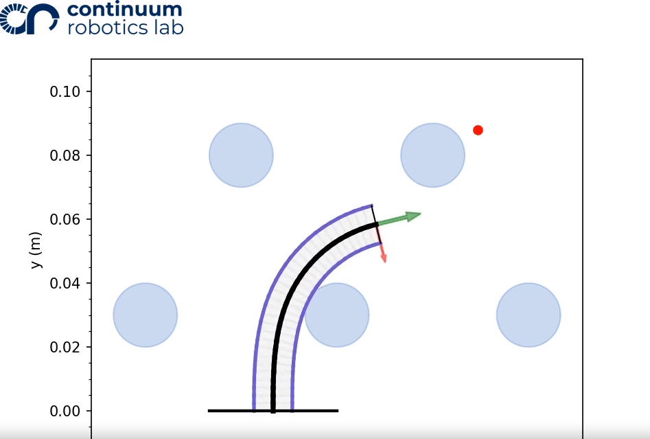
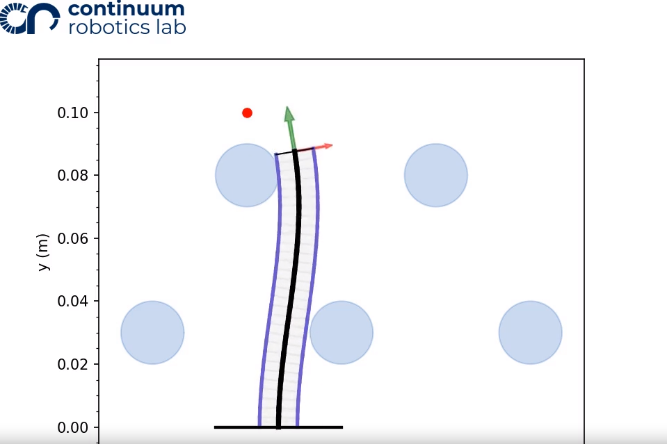
After the model has been run, and the nodes curvature values are determined, we can visualize the robot and taskspace by plotting it. The red dot is our target position.
config_init.plot_configuration(workspace)
helpers.saveFigure()
# plt.show()
Visualizing a Motion Plan
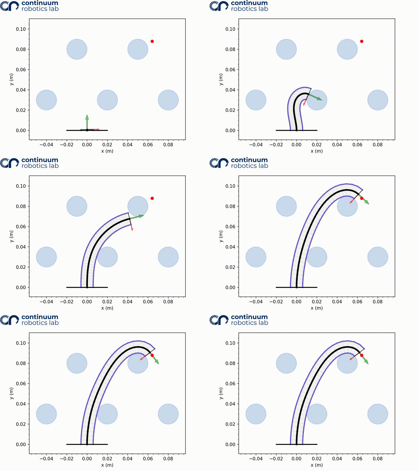
For every motion plan that is generated and simulated, it can be visualized as a mp4 video.
helpers.visualizing(traced_path, workspace, "filename")
Using the default taskspace and 3_sample_path.csv, the resulting video is:
Happy tendon driven continuum robotic simulating!
References
-
K.P. Ashwin, Soumya Kanti Mahapatra, Ashitava Ghosal: Profile and contact force estimation of cable-driven continuum robots in presence of obstacles. Mechanism and Machine Theory, 164:104404, 2021. doi: 10.1016/j.mechmachtheory.2021.104404 ↩
-
Priyanka Rao, Itai Spigelman, Oren Salzman, Jessica Burgner-Kahrs: Computationally Efficient Lookahead Search for Contact-aided Navigation for Tendon-driven Continuum Robots. CRL, 164:104404, 2024. pdf ↩ ↩2
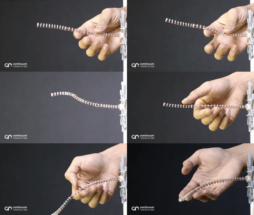
While changing the robot design mechanically is viable, we asked ourselves whether we can harness more from the traditional single segment straight routing design to achieve more variation than just a constant-curvature. What if these additional forces/moments came from the environment instead of mechanical additions - which would be possible if the robot now leveraged the obstacles to change its curvature? This idea inspired our research on contact-aided navigation for these robots.
Reaching a target
Let’s consider a single segment TDCR in a planar workspace, cluttered with obstacles marked in blue. If the robot tip needs to reach the target position (red dot in the animation below), it is a fairly simple task. You basically need to select actutation values that minimize the distance between the tip and the target. We can set up a simple joint space search for this - where we consider three possible actions:
- segment length increase (as its inserted into the workspace),
- tendon length decrease, and
- tendon length increase.
Starting from an initial joint value, these three actions can be sequentially applied to build a lattice-based representation of the configuration space.
A lattice is a discretization of the configuration space into a set of states, and connections between these states, where every connection represents a feasible path.3
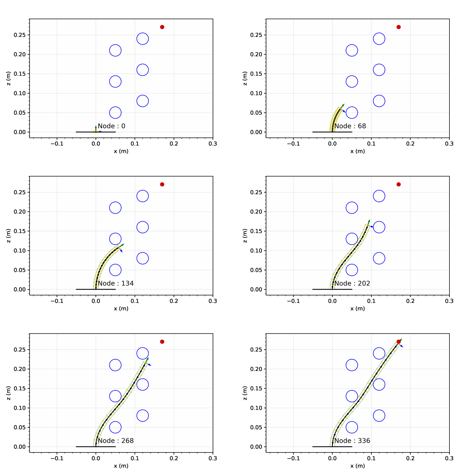
For now, lets keep optimality aside and focus on finding a solution by performing a greedy search. The greedy search is guided by a heuristic - for our case, we can set this heuristic to simply be the Euclidean distance between the robot tip and the target. This simple heuristic works quite well! There some additional changes you can make to prevent it from getting stuck in minimas but we will leave that discussion for another day.
Reaching a target pose
Now that we have a solution to reach a target position, we can add an additional layer of challenge to our problem - How can we reach a target, with not just the desired position, but a desired orientation as well? We can retain all the machinery from the previous section, of building a lattice in the configuration space by sequentially applying joint space actions. But the more important question we need to answer is:
What would the heuristic look like to reach a target pose?
To reach a desired pose, we need to control x, y, and theta of the tip. However, we only have two controllable degrees-of-freedom where we can either change the length of the segment or bend it. The single segment is essentially underactuated for this task - leveraging contact-aided navigation allows the segment to use the obstacle as a kind-of passive degree of freedom to control the tip.
Our work, recently published in the IEEE Robotics & Automation Letters4, seeks to solve this problem. The heuristic basically assumes that the end-effector’s motion can be modeled as a series of constant-curvature arcs - arcs whose end-points can only lie on the surface of obstacles. This condition ensures that the use of obstacles as a degree of freeodm is captured by the heuristic.
You can watch some of the solutions found by our method in the video below :
Open-Source materials
For now, we are releasing a preliminary version of the TDCR that can account for contacts on GitHub (link below). It is based on the kinematic model proposed by Ashwin et al. 5.
Please watch this space for more details and tutorials!
References
-
R.M. Grassmann, P. Rao, Q. Peyron, J. Burgner-Kahrs: FAS—A Fully Actuated Segment for Tendon-Driven Continuum Robots. Frontiers in Robotocs and AI, 9:873446, 2022. doi: 10.3389/frobt.2022.873446 ↩
-
P. Rao, C. Pogue, Q. Peyron, E. Diller, J. Burgner-Kahrs: Modeling and Analysis of Tendon-Driven Continuum Robots for Rod-Based Locking. IEEE Robotics & Automation Letters, 8(6):3126 - 3133, 2023. doi: 10.1109/LRA.2023.3264869 ↩
-
B. J. Cohen, G. Subramania, S. Chitta, M. Likhachev: Planning for Manipulation with Adaptive Motion Primitives. IEEE International Conference on Robotics and Automation, pp. 5478-5485, 2011. doi: 10.1109/ICRA.2011.5980550 ↩
-
P. Rao, O. Salzmann, J. Burgner-Kahrs: Towards Contact-Aided Motion Planning for Tendon-Driven Continuum Robots. IEEE Robotics & Automation Letters, 2024. doi: 10.1109/LRA.2024.3383211 ↩
-
K.P. Ashwin, Soumya Kanti Mahapatra, Ashitava Ghosal: Profile and contact force estimation of cable-driven continuum robots in presence of obstacles. Mechanism and Machine Theory, 164:104404, 2021. doi: 10.1016/j.mechmachtheory.2021.104404 ↩
In certain medical applications, physicians may want to inspect some region of interest for diagnostic purposes completing the procedure as fast as is safely possible to reduce costs and improve patient outcomes, especially if the patient is under anesthesia during the procedure. For example, the needle-diameter Continuum Reconfigurable Incisionless Surgical Parallel (CRISP) robot 1 2 was suggested to assist in the diagnosis of the cause of a pleural effusion (a serious medical condition that can cause the collapse of a patient’s lung) by visually inspecting the surface of the collapsed lung and chest wall inside the body3 (see Figure below).
Inspection Planning
This can modeled as an inspection-planning problem where we are given a robot equipped with a sensor and a set of points of interest (POI) in the environment to be inspected by the sensor. The problem calls for computing a minimal-length motion plan for the robot that maximizes the number of POI inspected.
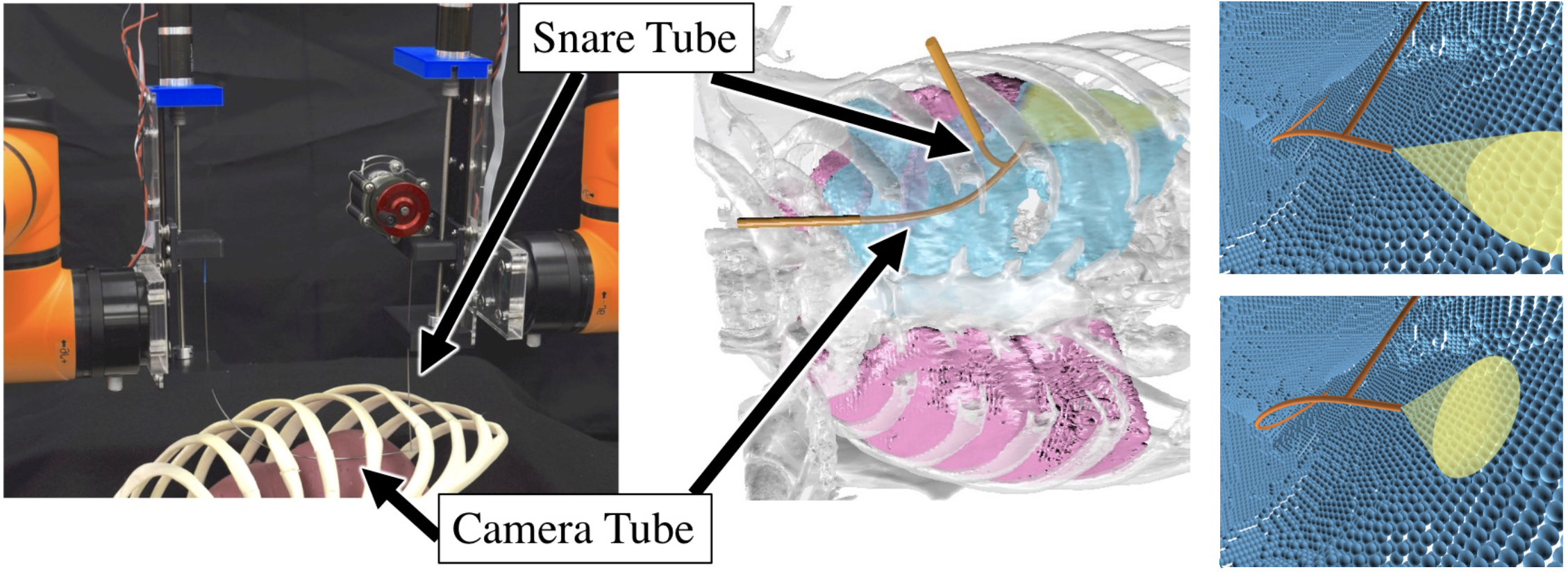
Naively computed inspection plans may enable inspection of only a subset of the POI and may require motion plans significantly longer than an optimal plan, and hence may be undesirable or infeasible due to time constraints. Our goal is to compute kinematically feasible collision-free inspection plans that maximize the number of POI inspected, and of the plans that inspect those POI we compute a shortest one.
What makes it challenging
Inspection planning is computationally challenging because we need to simultaneously reason both about motion planning in a high-dimensional configuration space (the space of all parameters that determine the shape of the robot) as well as about maximizing the number of POI inspected.
There are multiple approaches to computing inspection plans, but here we focus on those that provide some formal guarantee on the quality of the solution. Generally speaking these methods (see, e.g., 4 5) exhaustively search over the space of all motion plans thus guaranteeing asymptotic optimality. Roughly speaking, asymptotic optimality for inspection planning means these methods produce inspection plans whose length and the number of points inspected will asymptotically converge to those of an optimal inspection plan, given enough planning time.
Let’s dive deeper into the term we used earlier “exhaustively search over the space of all motion plans”. To do so, let’s go back to basics and consider shortest-path computation for a while (it may be worthwhile to visit previous posts on motion planning Part 1, Part 2). When we want to compute the shortest path to some point we can use the fact that any sub-path of a shortest path is also a shortest path. Namely, if we know that the shortest path between a and c passes through intermediate point b and we need to consider two paths connecting a and b, then the shorter one will always be better and we can discard the longer one. This is because if we take the shortest path connecting b and c it will always be preferable to append it to the shortest path connecting a and b. This is referred to as Bellman’s principle of optimality.
Going back to our problem of inspection planning this is not necessarily the case. To understand this, assume that we have two POIs and recall our two paths connecting a and b. Assume that the shorter one sees no POI while the longer one sees the first POI. Which one is better? We actually don’t know because it depends on the future: if we consider the first path, then we need to find a path between b and c that sees both POIs while if we consider the second path then we only need to find a path between b and c that sees the second POI.
To summarize, for each intermediate point, we need to consider the trade-off between short paths that see less POI and long paths that see more POI. This set has a name, “The Pareto-optimal frontier”. The set of Pareto-optimal inspection plans is the minimal set of inspection plans such that each plan is either shorter or has better coverage of the POI than any other inspection plan. Unfortunately, computing this set comes at the price of very long computation times as the size of the search space is exponential in the number of POI.
IRIS - Incremental Random Inspection-roadmap Search
To solve the slow running times of existing algorithms, we introduced a new algorithm which we called Incremental Random Inspection-roadmap Search, or IRIS, which is an asymptotically optimal inspection-planning algorithm 6 7. Similar to sampling-based planners1 2, IRIS incrementally constructs a sequence of increasingly dense roadmaps (graphs embedded in the configuration space) wherein each vertex represents a collision-free configuration and each edge a collision-free transition between configurations - and computes an inspection plan on the roadmaps as they are constructed.
Unfortunately, even the problem of computing an optimal inspection plan on a graph (and not in the configuration space) is computationally hard (see discussion above on computing the Pareto-optimal frontier). To circumvent this, we compute a near-optimal inspection plan on each roadmap. Basically, we use the fact that if two paths are “almost the same length” and see “almost the same set of POI”, essentially they are the same for all practical purposes and we can store only one (we have formal definitions for the “almost”s and the “essentially” but theses are out of the scope of this post).
This additional flexibility allows us to improve the quality of our inspection plan in an anytime manner, i.e., the algorithm can be stopped at any time and return the best inspection plan found up until that point. We achieve this by incrementally densifying the roadmap and then searching over the densified roadmap for a near-optimal inspection plan—a process that is repeated as time allows. By reducing the approximation factor (the mathematical tool we use to dictate which paths we consider paths as essentially the same) between iterations, we ensure that our method is asymptotically optimal.
This allowed us to demonstrate the efficacy of our approach in simulation for several complex robotic systems as demonstrated in the Figure above.
For additional details on algorithmic motion planning for continuum robots, see 8 and references within.
References
-
Arthur W Mahoney, Patrick L Anderson, Philip J Swaney, Fabien Maldonado, and Robert J Webster III. Reconfigurable parallel continuum robots for incisionless surgery. IEEE IROS, pp 4330–4336, 2016. doi: 10.1109/IROS.2016.7759637 ↩ ↩2
-
Patrick L Anderson, Arthur W Mahoney, and Robert J Webster III. Continuum reconfigurable parallel robots for surgery: Shape sensing and state estimation with uncertainty. IEEE Robot. Autom. Lett., 2(3):1617–1624, 2017. doi: 10.1109/LRA.2017.2678606 ↩ ↩2
-
Alan Kuntz, Chris Bowen, Cenk Baykal, Arthur W Mahoney, Patrick L Anderson, Fabien Maldonado, Robert J Webster III, and Ron Alterovitz. Kinematic design optimization of a parallel surgical robot to maximize anatomical visibility via motion planning. IEEE ICRA, pp 926–933, 2018. doi: 10.1109/ICRA.2018.8461135 ↩
-
Andreas Bircher, Kostas Alexis, Ulrich Schwesinger, Sammy Omari, Michael Burri, and Roland Siegwart. An incremental sampling–based approach to inspection planning: The rapidly–exploring random tree of trees. Robotica, 35(6):1327–1340, 2017. doi: 10.1017/S0263574716000084 ↩
-
Premysl Kafka, Jan Faigl, and Petr Vana. Random inspection tree algorithm in visual inspection with a realistic sensing model and differential constraints. IEEE ICRA, pp 2782–2787, 2016. doi: 10.1109/ICRA.2016.7487440 ↩
-
Mengyu Fu, Alan Kuntz, Oren Salzman, and Ron Alterovitz. Toward asymptotically-optimal inspection planning via efficient near-optimal graph search. In RSS, 2019. doi: 10.15607/RSS.2019.XV.057 ↩
-
Mengyu Fu, Alan Kuntz, Oren Salzman, Ron Alterovitz. Asymptotically optimal inspection planning via efficient near-optimal search on sampled roadmaps. The International Journal of Robotics Research, 42(4-5):150-175, 2023. doi: 10.1177/02783649231171646 ↩
-
Oren Salzman. Algorithmic Motion Planning Meets Minimially-Invasive Robotic Surgery. IJCAI,pp 7039-7044, 2023. doi: 10.24963/ijcai.2023/804 ↩
Steerable needles are a type of continuum robot, distinguished by their flexibility and capability to navigate through complex anatomical pathways. These robots are highly under-actuated, relying on interaction with the environment for movement and direction. The steering mechanism of steerable needles utilizes the asymmetric tip’s interaction with tissue forces during insertion. By externally rotating the needle shaft, the tip’s orientation is adjusted, allowing for controlled deflection towards desired directions upon further insertion. This method enables the needle to maneuver around obstacles such as bones, vessels, and nerves, accessing multiple targets without complete withdrawal. The reliance on environmental interaction for actuation not only enhances the safety and efficacy of medical interventions but also presents challenges and opportunities in motion planning and control within robotics, emphasizing navigation in environments with complex constraints and precision requirements.
Motion Planning for Steerable Needles
Steerable needles can be used to reach clinical targets for biopsy purposes while safely avoiding obstacles such as blood vessels. This clinical application can be modeled as a motion-planning problem which is the problem of determining a collision-free path or trajectory for a robot to move from its initial position to a desired goal position while avoiding obstacles in its environment (see also previous motion planning posts Part 1, Part 2).
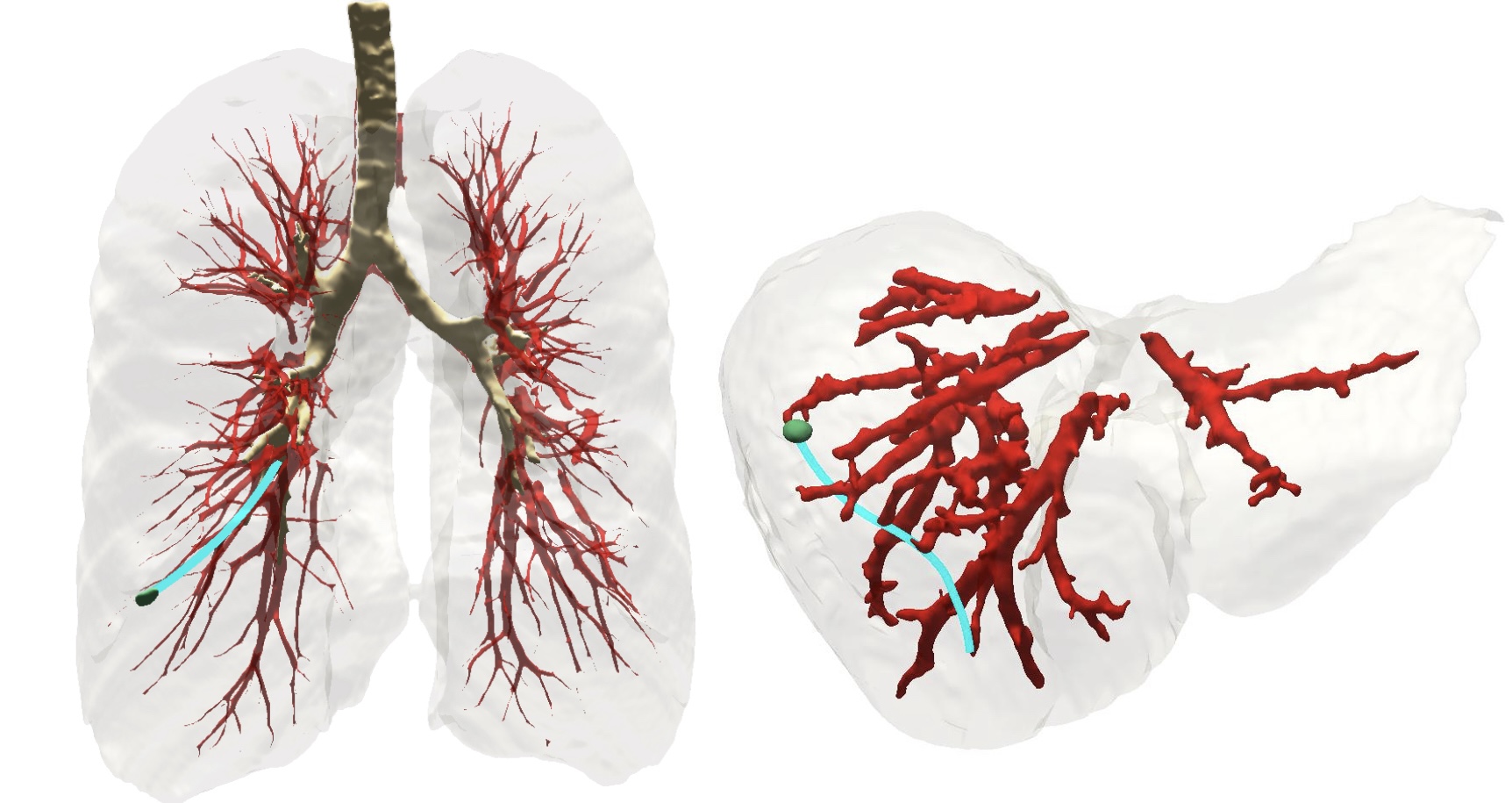
Ideally, a motion-planning algorithm should first guarantee that it will compute a solution, if one exists, in finite time, or notify the user that no solution exists (we call such motion planners complete”). Moreover, the computed solution should strive to maximize some objective which in our setting is patient safety (we call such motion planners optimal). This can be quantified using metrics such as minimizing trajectory length, maximizing the minimal distance from obstacles and minimizing damage to sensitive tissue (see, e.g., 1 2 3 4). Unfortunately, the lion’s share of planners developed for steerable needles offer no formal guarantee on completeness, let alone optimality.
Some prior motion planners for steerable needles (see, e.g, 5 6 7) do aim to optimize motion-plan cost but they lack global optimality guarantees (this means that the cost of the solution they return may be a local optima). Some sampling-based planners (see, e.g., 8 9) are known to be both complete and optimal but those properties are usually proven only when they number of samples they use approaches infinity (this is referred to as asymptotic optimality).
These challenges inspired us to consider variants of completeness or optimality relevant to medical applications: In a series of recent papers (see, 10 11), we focus on specific types of guarantees relevant to real-world medical applications: resolution completeness and resolution optimality. Generally speaking, a resolution characterizes the discretization of some space such as the action space or configuration space of a robot. An algorithm is resolution complete if there exists a fine-enough resolution with which the algorithm finds a plan in finite time when a qualified solution exists, and otherwise correctly returns that no such plan exists. An algorithm is resolution optimal if it is resolution complete and if, when it does return a motion plan, the plan’s cost is guaranteed to be within a desired approximation factor of the cost of a globally optimal qualified motion plan. We illustrate this in the Figure below with an example showing searches with different resolutions for needle steering.
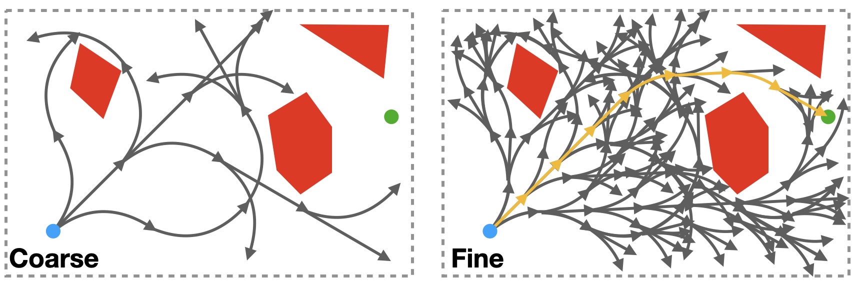
Resolution-Complete Search
We first presented Resolution-Complete Search (RCS), an efficient, resolution-complete motion planner for steerable needles based on a novel adaptation of multi-resolution planning 8. Under some mild assumptions on the system and the solution, the planner, in finite time, is guaranteed to find a plan as long as the problem admits a qualified solution. We then extended RCS to develop RCS*, that achieves resolution optimality 9.
We demonstrated the performance of our planners in two clinically realistic scenarios where the needle should reach a target while safely avoiding obstacles (e.g., blood vessels). In the setting of lung biopsy, where the needle is deployed through a bronchoscope and must steer through the lung parenchyma (the tissue of the lung outside the bronchial tubes) and in the setting of liver biopsy, where the needle is deployed into the liver through its anterior surface and must steer through the liver tissue. We compared in simulation our planner with several other steerable needle planners and demonstrated experimentally that RCS and RCS* outperform the state-of-the-art in terms of computation time, success rate, and plan quality.
For additional details on algorithmic motion planning for continuum robots, see 12 and references within.
References
-
Alberto Favaro, Leonardo Cerri, Stefano Galvan, Ferdinando Rodriguez Y Baena, and Elena De Momi. Automatic optimized 3D path planner for steerable catheters with heuristic search and uncertainty tolerance. IEEE ICRA, pp 9–16, 2018. doi: 10.1109/ICRA.2018.8461262 ↩
-
Alan Kuntz, Luis G Torres, Richard H Feins, Robert J Webster III, and Ron Alterovitz. Motion planning for a three-stage multilumen transoral lung access system. IEEE IROS, pp 3255–3261, 2015. doi: 10.1109/iros.2015.7353829 ↩
-
Mengyu Fu, Alan Kuntz, Robert J Webster III, and Ron Alterovitz. Safe motion planning for steerable needles using cost maps automatically extracted from pulmonary images. IEEE IROS, pp 4942–4949, 2018. doi: 10.1109/IROS.2018.8593407 ↩
-
Michael Bentley, Caleb Rucker, Chakravarthy Reddy, Oren Salzman, Alan Kuntz. Safer Motion Planning of Steerable Needles via a Shaft-to-Tissue Force Model. J. Medical Robotics Res. 8(1&2): 2350003:1-2350003:16, 2023. doi: 10.1142/S2424905X23500034 ↩
-
Jijie Xu, Vincent Duindam, Ron Alterovitz, and Ken Goldberg. Motion planning for steerable needles in 3D environments with obstacles using rapidly-exploring random trees and backchaining. IEEE CASE, pp 41–46, 2008. doi: 10.1109/COASE.2008.4626486 ↩
-
Sachin Patil, Jessica Burgner, Robert J Webster III, and Ron Alterovitz. Needle steering in 3D via rapid replanning. IEEE Trans. Rob., 30(4):853–864, 2014. doi: 10.1109/TRO.2014.2307633 ↩
-
Marlene Pinzi, Stefano Galvan, and Ferdinando Rodriguez y Baena. The adaptive hermite fractal tree (AHFT): a novel surgical 3D path planning approach with curvature and heading constraints. International Journal of Computer Assisted Radiology and Surgery, 14(4):659–670, 2019. doi: 10.1007/s11548-019-01923-3 ↩
-
Steven M LaValle. Planning algorithms. Cambridge university press, 2006. ↩ ↩2
-
Oren Salzman. Sampling-based robot motion planning. Commun. ACM, 62(10):54–63, 2019. doi: 10.1145/3318164 ↩ ↩2
-
Mengyu Fu, Oren Salzman, and Ron Alterovitz. Toward certifiable motion planning for medical steerable needles. In RSS, 2021. ↩
-
Mengyu Fu, Kiril Solovey, Oren Salzman, and Ron Alterovitz. Resolution-optimal motion planning for steerable needles. IEEE ICRA, pp 9652–9659, 2022. doi: 10.1109/ICRA46639.2022.9811850 ↩
-
Oren Salzman. Algorithmic Motion Planning Meets Minimially-Invasive Robotic Surgery. IJCAI,pp 7039-7044, 2023. doi: 10.24963/ijcai.2023/804 ↩
The idea is something I can relate to largely. Robotics Education is only just taking off in most parts of the world. With this project, I designed something that students at my home university, Manipal Institute of Technology in India, would be able to build. For the design, we considered various constraints such as component availability, 3D printer access, and skill level.
Components
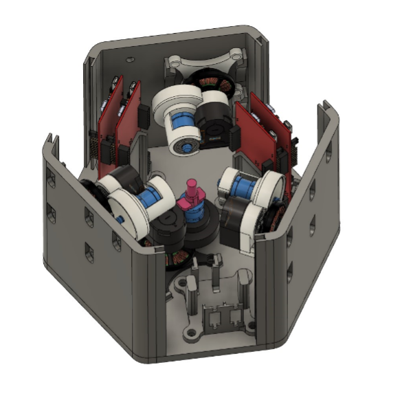
The kit comprises a Tendon Driven Continuum Robot (TDCR), four actuators, two TI Launchpads, various complementary electronic components, and a custom casing to enclose the entire system. For the sake of brevity, I have omitted details thoroughly explained on our GitHub.
Manipulator
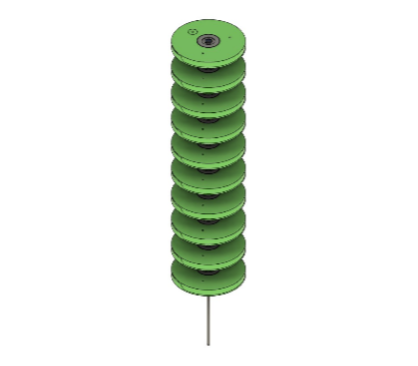
The manipulator of the TDCR consists of 10 Type-II spacer disks equally distributed along a Nitinol Backbone with a diameter of 1.4 mm. The robot is capable of 3 DOFs, namely bending across two planes and rotation about its axis. I used three independently actuated tendons made of Spectra Fiber and an actuator to rotate the backbone, enabling these degrees of freedom.
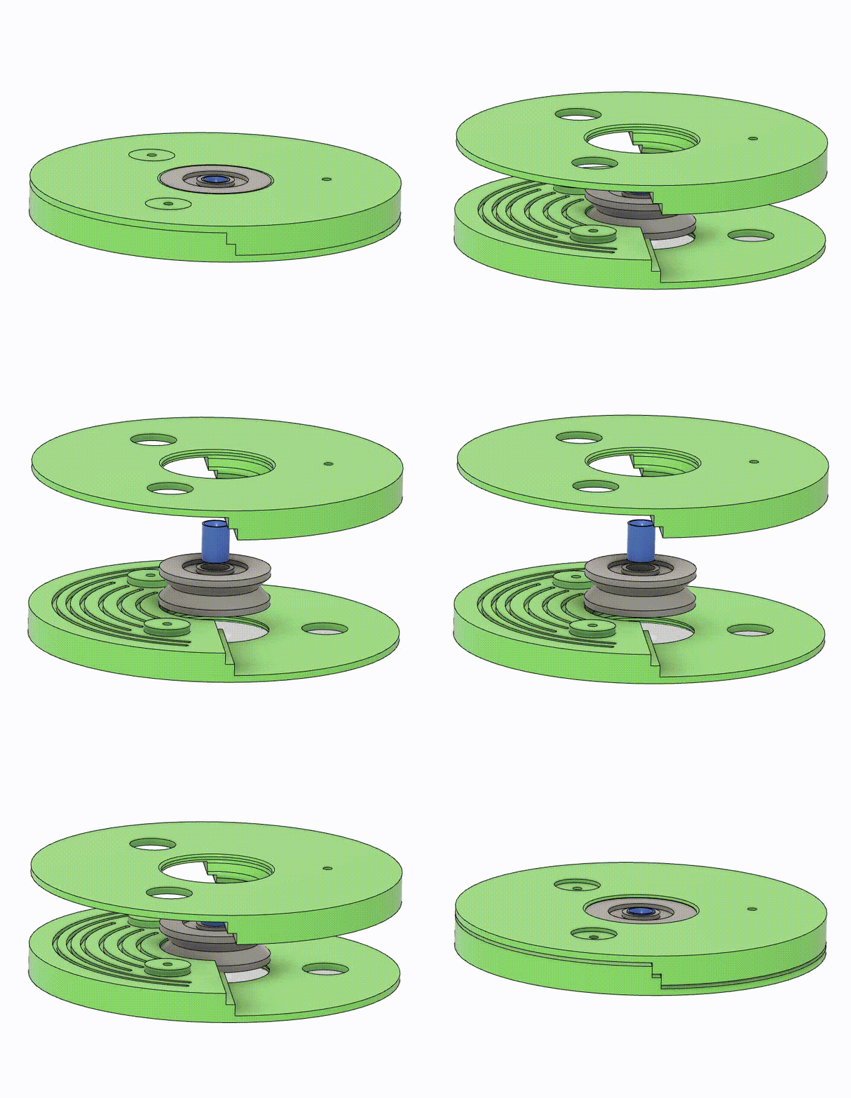
The body of the spacer disk is fixed to the backbone axially, while a bearing in the middle enables the rotational DOF. It is split into two parts to allow for the insertion of the bearing in the middle. I changed the regular ball bearing to a pulley to reduce the number of unique components. The profile of the two parts allows for easy assembly while ensuring that the actuation through the tendons is optimal. The grooves ensure the adhesive stays inside the segment and does not spill out. A small part, functioning as a spacer to make the pulley bore smaller, is designed with a unique profile that balances the required friction to grip the backbone and the need for a constant curvature.
 |
 |
 |
Actuators
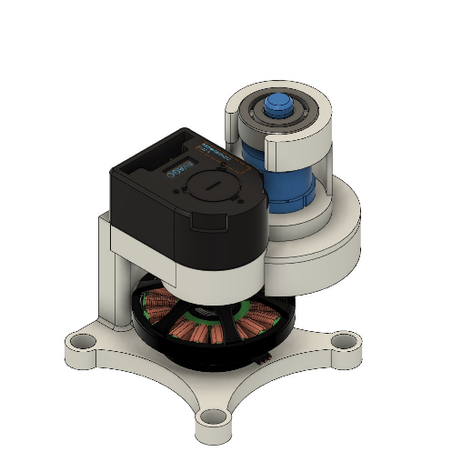
Our actuation module was modified to suit this kit’s requirements. I replaced the multi-part casing with a single unit, such that the new case is easier to manufacture while maintaining adequate performance. The assembly process is simplified as the singular casing eliminates input and output shaft misalignment. The motor and the gears can easily fit into designated spaces using dedicated slots. Since the actuator will only actuate tendons, I introduced an extra bearing at the output shaft to handle the increased radial tension and eliminate shaft eccentricity.
I used the Launchpad TI LAUNCHXL-F28069M, a microcontroller development board, to control the motors with two motor Drivers, BOOSTXL-DRV8305EVM. Since four motors and each motor driver can control one motor, two Launchpads and four motor drivers are required to actuate the continuum robot.
 |
 |
Housing
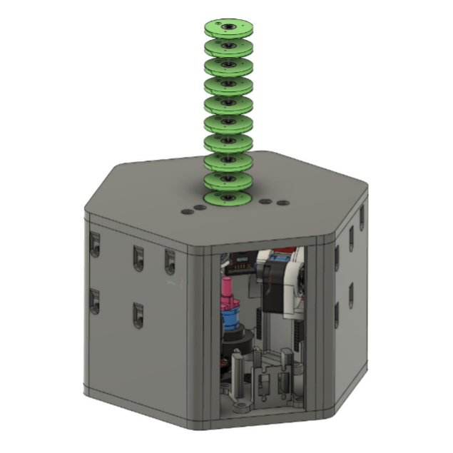
All components are placed inside a hexagonal casing with windows made of transparent acrylic sheets to view the system’s working. The three tendon actuators are fixed horizontally to reduce tendon routing. Six pulleys are placed inside to help reduce the tendon offset and increase the efficiency of tendon control. One actuation module is placed at the bottom and controls backbone rotation. To secure the electric components in the case, I designed custom 3D-printed mounts. All components are visible from the windows to allow the user to see the robot’s functioning, allowing better understanding and enabling intuition development.
I used several techniques to adapt the design for manufacturing with an FDM 3D Printer:
- teardrop method to ensure optimal vertical holes
- eliminated 90° overhangs using arcs
- used chamfers to reduce support material.
- counterbores for all bolt heads ensure a flush surface finish on all casing sides
- included partial slots for nuts to make assembly easier
Assembly Guide
Find a detailed assembly guide, printable STL Files and mechanical drawings on GitHub and watch the assembly video on YouTube: GitHub Video
I encourage you to try and fabricate this learning kit and contact us regarding any queries or further developments you make! We would love to hear about your experience and see your prototypes!
Epilogue
I took the design home and encouraged robotics enthusiasts at my home university to build and use OpenCR’s Learning Kit. The learning kit allows students to easily understand concepts, design, and implement various algorithms. I hope this kit or its successor will find its way into classrooms at different schools! Stay tuned for updates.
References
-
Reinhard M. Grassmann, Priyanka Rao, Quentin Peyron, Jessica Burgner-Kahrs: FAS — A Fully Actuated Segment for Tendon-Driven Continuum Robots. Front. Robot. AI 9:873446, 2022. doi: 10.3389/frobt.2022.873446 ↩
-
Reinhard M. Grassmann, Chengnan Shentu, Taqi Hamoda, Puspita Triana Dewi, Jessica Burgner-Kahrs. “Open Continuum Robotics – One Actuation Module to Create them All,” 2023, arXiv: 2304.11850 ↩
What makes motion planning particularly challenging for continuum robots?
First, let’s discuss one of the primary differences between continuum robots and more “traditional” robots (for lack of a better term)—modeling.
As you’ve seen in prior (and future, I promise) blogs on this site, modeling the mechanics of continuum robots is fundamentally different from more traditional serial-link manipulator arms.
As a subset of mechanics, consider just the forward kinematics (FK) problem for continuum robots, i.e., mapping the robot’s joint state to the robot’s resultant shape in space. For concentric tube robots this may be mapping the robot’s tubes’ rotation/translation values to the robot’s shape and for tendon-driven robots this may be mapping the robot’s tendon tensions/displacements to the robot’s shape.
What’s actually happening in the physical world is complicated here. There are elastic elements interacting with (potentially) other elastic elements in complex ways. There is difficult-to-model friction between components of the robot, hysteresis, potentially difficult-to-predict material properties, etc.
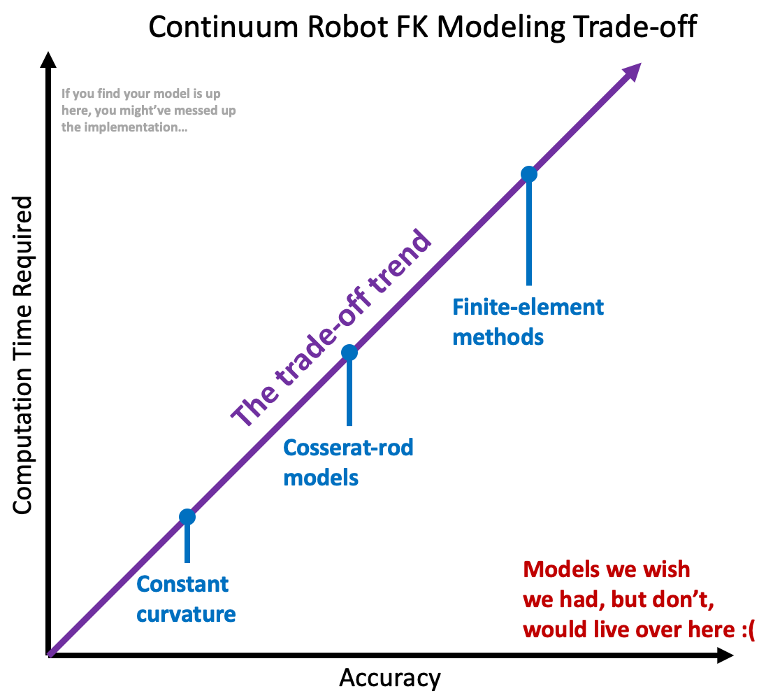
The continuum robotics community has taken a variety of approaches to modeling, but a fundamental trend exists: a trade-off between accuracy and speed-of-computation. That is, models which may be fast to compute are typically fast because they neglect to account for some of the physical phenomenon present in the actual robot. On the flip side, models that account for those phenomenon are slow to compute. In reality, there’s a spectrum here.
Constant curvature models, for instance, may take a purely geometric approach to FK, which is fast to compute, but tend to be less accurate. On the other end of the spectrum, you could consider leveraging something like finite element analysis to simulate the physics of a continuum robot to compute its shape. This would improve accuracy but would be much, much slower to compute. Somewhere in the middle of these you may find things like the Cosserat rod/string models, which are a popular way to model continuum robots and will be discussed in other blog posts here (this is the approach we take in my lab, usually, when we aren’t using machine learning-based methods).
Let’s contrast this with serial-link manipulator arms. For these, FK typically require only the multiplication of a handful of matrices, which is comparatively VERY fast, and comparatively VERY accurate, as these robots are rigid.
Okay, so why is this a problem when performing motion planning for continuum robots?
Well, one way to think about motion planning is that we are reasoning in advance of actually moving about the best way to move the robot to achieve our goals. This means that we need our ability to reason about motion to be accurate, otherwise how we predict the robot will move doesn’t mean much. For this reason, model inaccuracy plays havoc with naïve motion planning methods (such as we’ve discussed in last week’s post), and continuum robots have inaccurate models.
Further, the ways in which we are reasoning in advance about moving require us to consider a whole bunch of potential motions for the robot. Every vertex in the grid/lattice-based and sampling-based methods represents an FK computation. Every edge between them requires multiple (often many) FK computations. In the optimization-based methods, the computation of objective and constraint gradients frequently require many FK computations. So the time it takes to compute FK has HUGE implications in motion planning.
This modeling tension, fast but inaccurate or (somewhat) accurate but slow, is one of the fundamental challenges of applying motion planning to continuum robots, and the one I’ll focus on for the rest of this post.
How has the community overcome these challenges?
Modeling accuracy (or lack thereof)
The continuum robotics community (myself included) has largely taken an extremely unsatisfying approach to overcoming modeling inaccuracy. This approach, also used by much of the non-continuum robotics planning world, boils down to a simple idea: don’t let the robot get close to things. That way, if the model is inaccurate, hopefully the robot is far enough away from its environment that it won’t collide with it in unexpected ways.
As an example, in one of my papers1, we build into the objective function a notion of distance from obstacles. Specifically, We define the cost of a configuration $\boldsymbol{q}$ as:
\[\begin{split} &\texttt{cost}(\boldsymbol{q})=\left\{ \begin{array}{rcl} \cfrac{1}{\texttt{clear}(\boldsymbol{q})},&&\texttt{clear}(\boldsymbol{q}) > 0\\ \infty,&&\texttt{clear}(\boldsymbol{q}) \le 0, \end{array}\right. \end{split}\]where $\texttt{clear}$ is, informally defined here, the signed distance from the robot’s body at that configuration to the nearest obstacle.
The cost of a path $\boldsymbol{\xi}$ then becomes \(\texttt{Cost}(\boldsymbol{\xi}) = \int_0^1 \texttt{cost}(\boldsymbol{\xi}(s))ds .\)
where $s$ is a normalized path arclength parameter. Note here that I’ve used little ‘c’ cost for cost over configuration and big ‘C’ Cost for cost over a path. Creative, I know.
You should really read the paper if you want formality here, but this should give you the gist. Also note that in the paper the notation is slightly different, but I’ve changed it here to more-closely match what I’ve used in the last post.
In that method, we leverage both sampling-based motion planning and optimization-based motion planning in parallel (building on [13]), where the method attempts to minimize the $\texttt{cost}$ of a path. This results in paths that travel as far from obstacles as possible, while still being constrained at the start and end configurations.
Computation speed (or lack thereof)
The community has taken a variety of approaches to overcome the slow computation speed of continuum robot mechanical models. Here are a few, with some examples.
The first, and most obvious, is the use of a fast-but-inaccurate mechanical model: For instance, in Lyons et al. 2, the authors simplify the mechanical model of concentric tube robots in two key ways. First, they assume that the tubes are torsionally rigid. Second, they assume that the stiffness of each tube dominates all of the tubes nested inside of it. This means that the shape of a tube is assumed to be independent of the motions of the tubes internal to it and that each tube deploys in a constant-curvature circular shape. The mechanical model that leverages these assumptions is sufficiently fast for planning, but again as discussed above ad nauseam, comes at the significant cost of accuracy.
Another approach is to lean on advances in software engineering and programming languages to speed up the computation: Leibrandt et. al.3 leverage template metaprogramming in C++, which (I’m oversimplifying this explanation) moves a lot of expensive run-time computation to compile-time computation for concentric tube robots. This enabled very fast kinematics computation. The method leverages this in a PRM-style motion planner. In our paper1 mentioned above, we use this template-based kinematic model, wrapping our parallel sampling and optimization method around it. Speaking of, our1 use of parallelism is another example of leveraging software engineering concepts to speed up computation in planning for continuum robots.
We can also consider leveraging precomputation: In the paper 4 (its extension 5), the authors propose leveraging precomputation to build a roadmap for planning after the environment is known but in advance of when it is needed. This is a pretty specific (and restrictive) scenario, but makes sense in the application put forth by the papers, namely in surgery. These works present the case that pre-operative medical imaging provides the method with a 3D environment a day (or more) prior to when the surgery will happen. The method can then leverage that time to compute a dense, collision-free roadmap before it’s needed at surgery time. The proposed method utilizes the sampling-based method Rapidly-exploring Random Graph (RRG) (which is also presented in 6, in addition to PRM* and RRT*). The method also utilizes one of, if not the most precise (at the time, at least) mechanical models available for concentric tube robots. This dense, collision-free roadmap is built over the course of many hours using this accurate model and the anatomical environment segmented from the pre-operative medical imaging. Then, at the time of the surgery, the method proposes an interactive-rate supervisory control-style scheme in which a haptic device is used by the surgeon to input a desired tip position for the robot in the patient. Leveraging a nearest-neighbor data structure, the vertex in the roadmap that corresponds to the configuration with the robot’s tip closest to the desired position is then identified. Graph search is performed to identify a path on the roadmap from the current configuration to that configuration, and then the method “steps off” of the roadmap and leveraging damped least-squares iterative inverse kinematics 78, which is conceptually very similar to resolved-rates control, drives the tip of the robot as close to the desired tip position as it can. This then repeats in a loop.
In our paper9, my group has built upon this concept in a few ways. Among other contributions, we adapt the concepts to work for tendon-driven continuum robots (4 and 5 are specific to concentric tube robots), introduce a modification to mechanical modeling and collision detection to improve speed, and remove the need to have the environment in advance of precomputing the dense roadmap. The method still heavily leverages precomputation, but only requires the environment immediately prior to when the supervisory control loop is started.
So what’s next?
What are the open problems or areas to be explored in motion planning for continuum robots? Here are a few that I’m personally excited about.
Leveraging learned models in planning
There has recently been a large interest in machine learning-based mechanical models of continuum robots, both for their potential to learn unmodeled (or unknowable/unmodelable) effects and their potential for fast computation (e.g., frequently the shape computation of a learned model is faster than the physics-based equivalent). I’ll leave the details of these methods to another post, written by myself or someone else. However germane to THIS post, how to leverage these types of models for motion planning of continuum robots is as-yet underexplored.
Principled planning under uncertainty
Motion planning in a way that handles uncertainty in a principled way has been leveraged to great effect in other areas of robotics. Given the uncertainty associated with continuum robots, the application/exploration of using these types of methods/formulations in planning for continuum robots has great potential.
Multi-fidelity planning
The fact that we have a variety of models for continuum robots that trade computation speed for accuracy implies exciting potential for the use of multi-fidelity planning. One can imagine, as maybe the most obvious example, using a fast but inaccurate model to prioritize edge evaluation in a lazy planning paradigm, look up Lazy PRM if that doesn’t make sense to you, where full edge evaluation is then done with a high-fidelity model.
Closing remarks
Hopefully the above alongside last week’s Part 1 were a relatively gentle introduction to motion planning and how it relates conceptually to continuum robots. This wasn’t intended to be a comprehensive survey of planning for continuum robots. Rather, my intention was to give you the vocabulary and an understanding of the rough concepts sufficient for you to investigate the rest of the literature yourself, and to innovate on the state-of-the-art as you need for your specific problems.
References
-
A. Kuntz, M. Fu, R. Alterovitz: Planning High-Quality Motions for Concentric Tube Robots in Point Clouds via Parallel Sampling and optimization. IEEE/RSJ International Conference on Intelligent Robots and Systems (IROS), pp. 2205-2212, 2019. doi: 10.1109/IROS40897.2019.8968172 ↩ ↩2 ↩3
-
L. A. Lyons, R. J. Webster, R. Alterovitz: Motion planning for active cannulas. IEEE/RSJ International Conference on Intelligent Robots and Systems, pp. 801-806, 2009. doi: 10.1109/IROS.2009.5354249 ↩
-
K. Leibrandt, C. Bergeles, G.-Z. Yang: Concentric Tube Robots: Rapid, Stable Path-Planning and Guidance for Surgical Use. IEEE Robotics & Automation Magazine, vol. 24, no. 2, pp. 42-53, 2017. doi: 10.1109/MRA.2017.2680546 ↩
-
L. G. Torres, C. Baykal, R. Alterovitz: Interactive-rate motion planning for concentric tube robots. IEEE International Conference on Robotics and Automation (ICRA), pp. 1915-1921, 2014. doi: 10.1109/ICRA.2014.6907112 ↩ ↩2
-
L. G. Torres et al.: A motion planning approach to automatic obstacle avoidance during concentric tube robot teleoperation. IEEE International Conference on Robotics and Automation (ICRA), pp. 2361-2367, 2015. doi: 10.1109/ICRA.2015.7139513 ↩ ↩2
-
S. Karaman and E. Frazzoli: Sampling-based algorithms for optimal motion planning. The International Journal of Robotics Research, 30(7):846-894, 2011. doi: 10.1177/0278364911406761 ↩
-
Y. Nakamura and H. Hanafusa: Inverse Kinematic Solutions With Singularity Robustness for Robot Manipulator Control. ASME. J. Dyn. Sys., Meas., Control., 108(3):163–171, 1986. doi: 10.1115/1.3143764 ↩
-
C. W. Wampler: Manipulator Inverse Kinematic Solutions Based on Vector Formulations and Damped Least-Squares Methods. IEEE Transactions on Systems, Man, and Cybernetics, 16(1):93-101, 1986. doi: 10.1109/TSMC.1986.289285 ↩
-
M. Bentley, C. Rucker, A. Kuntz: Interactive-Rate Supervisory Control for Arbitrarily-Routed Multitendon Robots via Motion Planning. IEEE Access, vol. 10, pp. 80999-81019, 2022. doi: 10.1109/ACCESS.2022.3194515 ↩
Motion planning stands as a central pillar in robotics. Planning enables robots and autonomous agents to move themselves and other parts of the world to a desired goal by choosing a sequence of appropriate actions. Like robotics in general, motion planning draws on a number of different fields in developing its tools. Approaches to motion planning have grown out of artificial intelligence, optimal control, and operations research.
That’s the first paragraph of my motion planning course syllabus. It’s a bit… grandiose, but I’ve found it to be effective in convincing the students that they are about to learn something interesting; hopefully it worked on you as well. It was also written by the professor who taught the course before I did, and whose syllabus I used as a starting point for my own (on the shoulders of giants etc etc etc). If that was sufficiently dramatic and you’re convinced to keep reading, let’s get to it.
More colloquially, motion planning can be broadly defined as the problem of computing motions, actions, or controls that move a robot through its environment in such a way that some task is performed while obeying some set of constraints.
In its most basic form, that task can be defined as moving from some start configuration to some goal configuration, with typical constraints being defined as obstacle avoidance over the motion, obeying joint limits, etc. Complexity in task definitions and constraint definitions builds from there.
I personally like to present motion planning as a generic optimization problem and then look specifically at how aspects of that problem are defined. Be forewarned, I’m going to grossly abuse notation/terminology and ignore nuance all over this post with the goal of imparting intuition rather than specifics.
Consider:
$\boldsymbol{\xi}^* = \underset{\boldsymbol{\xi}}{\texttt{argmin}}\ \texttt{cost}(\boldsymbol{\xi})$
$s.t. \ \ \ c(\boldsymbol{\xi}) \ge 0$ $\ \ \ \ \ \ \ \ d(\boldsymbol{\xi}) = 0$
where $\boldsymbol{\xi}$ represents some trajectory, path, or plan parameterization, $\texttt{cost}$ is some cost function defined over these, $\boldsymbol{\xi}^*$ is an optimal plan under the cost function, and $c$ and $d$ are generic, as-of-yet-unspecified inequality and equality constraints (or sets of such constraints).
This generic optimization formalization is sufficiently expressive to talk about most of the basics of motion planning, and by varying how aspects of this formalization are defined we can arrive at most of the ways people have historically thought about motion planning.
As an example, let’s consider the very simple (relative to other motion planning problems) task of moving a holonomic robot from some start state to some goal state while avoiding some set of obstacles in its environment.
If we conceptualize $\boldsymbol{\xi}$ as defining a space curve in the robot’s configuration space, we can parameterize $\boldsymbol{\xi}$ by the normalized path length such that $\boldsymbol{\xi}(0)$ is the robot’s start configuration and $\boldsymbol{\xi}(1)$ is the robot’s configuration after following the full plan.
Often people consider minimizing path length, so we can imagine defining $\texttt{cost}$ as the length of the path (under some appropriate definition of length).
We also want to constrain the trajectory such that the robot ends in a goal configuration (broadly as an element of some goal set), and such that the entire trajectory avoids obstacles.
We can then cast this simple problem into our optimization framework simply as:
$\boldsymbol{\xi}^* = \underset{\boldsymbol{\xi}}{\texttt{argmin}}\ \texttt{length}(\boldsymbol{\xi})$
$s.t. \ \ \ \boldsymbol{\xi}(0) = \textrm{start configuration}$
$\ \ \ \ \ \ \ \ \boldsymbol{\xi}(1) \in \textrm{goal set}$
$\ \ \ \ \ \ \ \ \boldsymbol{\xi}(s) \textrm{ is collision free } \forall s \in [0,1]$
As in most interesting things, key considerations lie in the details (which I’ve completely ignored above). How is your trajectory parameterized? How do you define your goal set? How do you represent your robot and environment geometry, enabling you to check for collision? Is length even the right objective to minimize? The answer to these questions depends on your specific problem/robot/etc. If I knew what this is for you, I’d just solve your problems myself and take all the credit.
Okay, so this is the first step—representing your problem. Next, let’s solve it.
How do methods typically work?
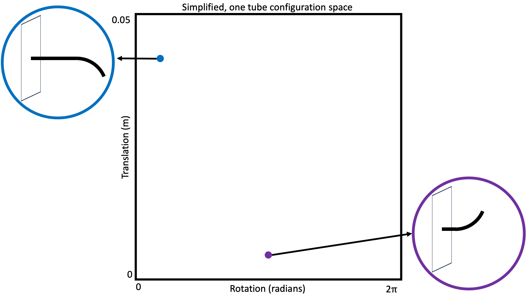
In my head I broadly group modern motion planning methods into three groups, discrete grid/lattice-based search methods, sampling-based methods, and optimization-based methods. There’s an implied fourth group, “other” or maybe “miscellany”, but I’m going to focus on the first three in this post.
Discrete grid/lattice-based search methods
At their simplest, these methods consider a graph or tree (which is just a special kind of graph) embedded in the robot’s configuration space. If you are unsure what I mean by “graph or tree” stop now and read this and this before moving on.
Notably for these methods, the graph is usually implied by a discretization over the robot’s possible actions. Imagine vertices of the graph as representing configurations or states of the robot, and edges as actions between states, which when applied from the source state result in the robot transitioning to the destination state. This action discretization is frequently defined in advance (and you can imagine applying this concept to robot’s with continuous action spaces simply by discretizing those action spaces). Due to the constant discretization, you can conceptualize these as creating something like a grid or lattice as the graph.
With this conceptualization, motion planning then reduces to a search over that graph, seeking the “shortest” path from your start vertex to any vertex that represents a goal configuration or state.
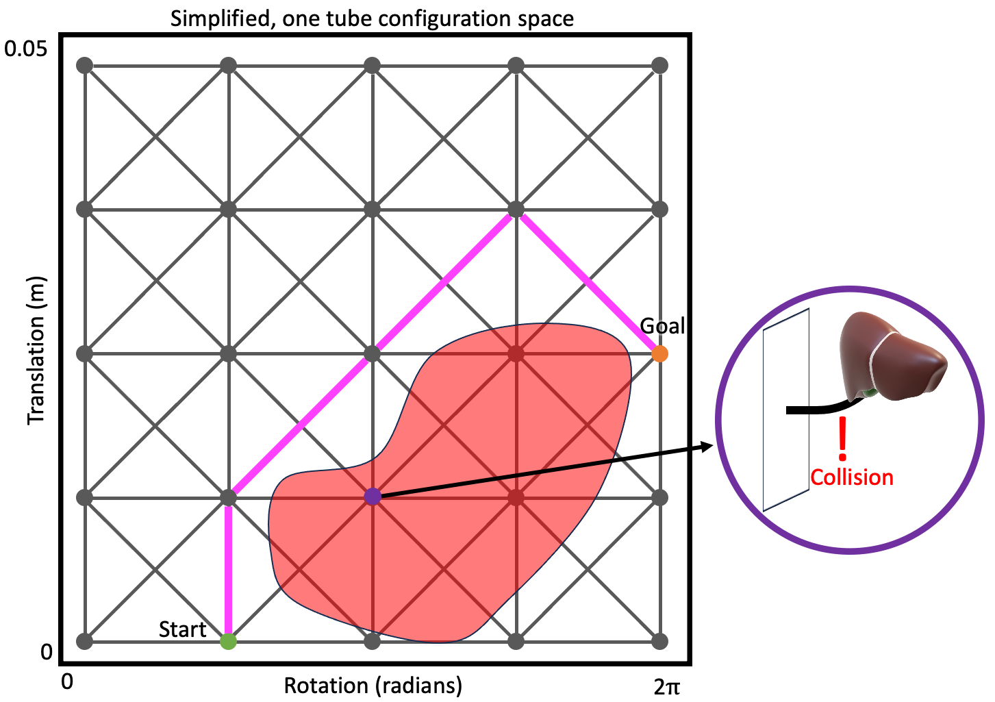
How does this map back to our optimization formalization above? The cost function is minimized by applying a graph-search method that minimizes the accumulation of edge cost (so you need to define a cost over edges and recognize that without substantial modification you’re limited to considering objectives that can be modeled by costs that accumulate). The constraints are enforced simply by not considering edges that would result in a violation of the constraints during the search.
Cannonical graph search methods (not specific to motion plannning) include Uniform Cost Search (UCS) (closely related to Djikstra’s algorithm) and A* search.
The key to applying these methods in motion planning is frequently in coming up with an effective and admissible/consistent heuristic (see A* details for what that means). More advanced methods applied to motion planning specifically include D*1, D*-Lite2, and LPA*3. It’s also very much worth noting that inadmissible heuristics can also be leveraged to potentially great effect (see Multi-Heuristic A*4).
Sampling-based methods
Perhaps the most popular class of motion planning methods, the sampling-based approaches are closely related to the graph-search methods. In fact, these methods frequently leverage graph search but on a graph constructed in a different manner.
Rather than a graph constructed via a discretization over the robot’s actions, the sampling-based methods leverage random sampling to construct the graph incrementally (this is why they are called sampling-based, as you may have guessed). The graph (or tree, which again, is just a special kind of graph) is embedded in the robot’s configuration space as above. It is constructed by iteratively randomly sampling states (or actions, sometimes) and attempting to connect the newly sampled state (or state resulting from the sampled action) to the graph/tree.
When adding states, (usually) the new state and the edge connecting it to the graph are checked for validity (e.g., joint-limit satisfaction and obstacle avoidance). If the state and/or edge are not valid, they aren’t added to the graph.
At some point, the hope is that the graph will contain a goal state, and then by running graph search (e.g., A*) on this randomly-generated graph the method will find a path from the start state to a goal. If the graph is a tree, this search is trivial as there’s only one path in the graph (ignoring some nuance, that’s what tree means).
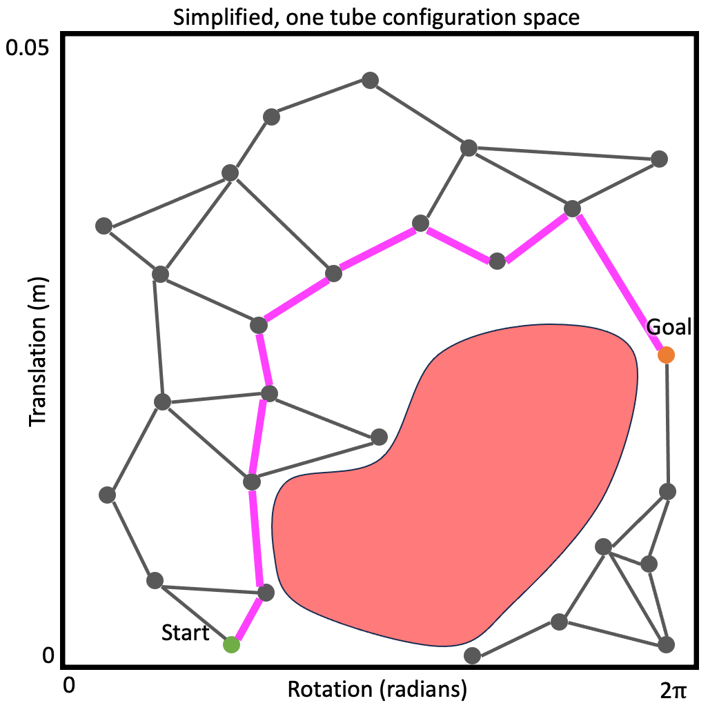
The specifics of the graph, how the states/actions are sampled, how the connections are made, etc., are what distinguish the sampling-based methods from each other.
Okay, so let’s map these concepts back to our optimization formulation.
Cost: If there are multiple paths in the graph, then the graph search over the graph can provide the lowest cost path in the graph, however the lowest cost path possible may not be in the graph at any given iteration. Many of the earlier versions of these methods ignored cost and instead attempted to find any path that avoided obstacles, providing a property called probabilistic-completeness. Since then, other methods build upon this to provide a guarantee called asymptotic optimality, which intuitively means that their best path will approach an optimal path (in cost) as runtime progresses (only getting arbitrarily close to an optimal path in the limit though). This contrasts with the discrete grid/lattice-based search methods in that those methods typically only provide a property called resolution completeness/optimality which intuitively means the path is complete or optimal for the resolution of the discretization, but not necessarily in general.
Constraints: As with the discrete grid/lattice-based search methods, the sampling-based methods usually encode constraint satisfaction by only considering states/edges in the graph construction or search that satisfy the constraints, including obstacle avoidance.
Canonical probabilistically-complete methods include Probabilistic Roadmaps (PRM)5 and Rapidly-exploring Random Trees (RRT)6. Popular asymptotically-optimal methods include PRM*/RRT*7, Batch-Informed Trees (BIT)8, and Asymptotically-Optimal-RRT (AO-RRT)9.
Super-duper important point! Just because you’re using sampling-based methods does not mean you’re getting probabilistic completeness or asymptotic optimality. There are properties/assumptions you must satisfy in your specific application of these methods that are frequently nuanced, you’ll need to ensure that you satisfy these things. Read the papers detailing these methods for details!
Optimization-based methods
Given the formulation we started with, i.e., casting the motion planning problem as constrained optimization, you may be asking yourself: “wait, why don’t we just use optimization methods from, you know, mathematics, to solve this problem?” Great question! Enter the optimization-based motion planning methods.
This class of methods leverages nonlinear, constrained optimization methods from the field of optimization itself explicitly to solve the motion planning problem using variations of our above formulation—rather than relying on the graph-search to minimize cost.
As of now, the majority of these methods (with an exception mentioned below) leverage gradients (and frequently higher-order derivatives) of the objective function and/or of the constraint functions in iterative optimization methods. Think penalty methods, augmented Lagrangian methods, interior point methods, etc. If these concepts are new to you, there is an amazing textbook on the subject by Wright and Nocedal 10 that is open almost perpetually in my office.
At a high level there isn’t much more to the story. These methods take exactly the optimization-based formulation above and apply optimization techniques that work directly on such formulations.
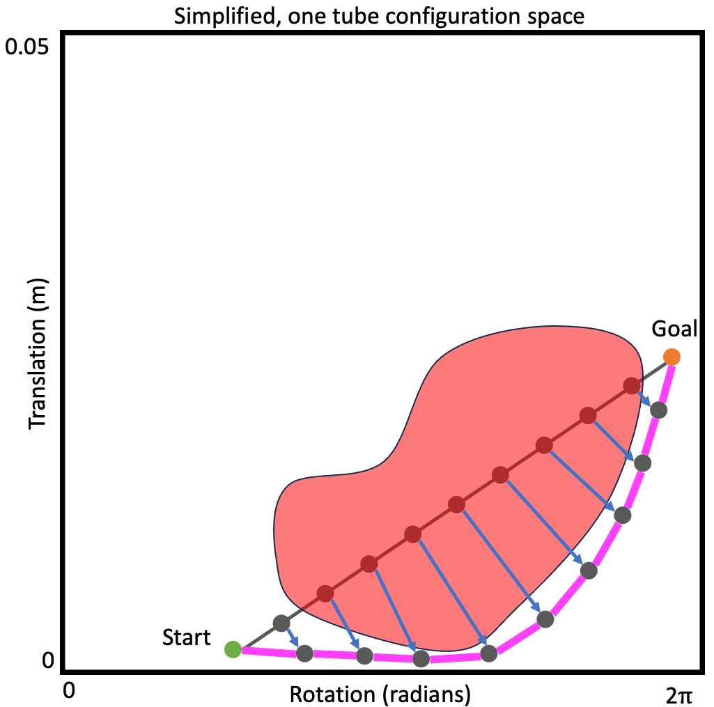
Is it just that easy? Unfortunately, no. The prior paragraph is true at a high level, but the low level is where the details lie. The specific ways in which these methods define cost and their constraint functions such that they work well with the optimization techniques—e.g., ensuring they have gradients that are well-behaved—can make these methods a bit tricky to use in practice. However in many cases they end up working very, very well, which can make it worth the complexity.
Canonical methods include CHOMP11, which leverages a variation of gradient descent, and TrajOpt12 which leverages Sequential Quadratic Programming (SQP). A different method, that is not nearly as popular as those methods, combines sampling-based planning with interior point optimization13. I include it in this list because it was part of yours truly’s PhD work, and so here is a shameless plug.
There is also a method called Cross-Entropy Motion Planning (CEMP)14 that leverages a gradient-free optimization method (the cross-entropy method, as you may have guessed from the name). This is notable because many difficulties one may encounter in leveraging optimization-based methods may come from the gradients, or lack-thereof.
This concludes Part 1 of my introduction to motion planning for continuum robots. In next week’s Part 2 we will look at the challenges of motion planning for continuum robots. Stay tuned!
References
-
A. Stentz: Optimal and Efficient Path Planning for Partially-Known Environments. IEEE International Conference on Robotics and Automation, pp: 3310–3317, 1994. doi: 10.1109/ROBOT.1994.351061 ↩
-
S. Koenig, M. Likhachev: Fast Replanning for Navigation in Unknown Terrain. Transactions on Robotics, 21(3):354–363, 2005. doi: 10.1109/tro.2004.838026 ↩
-
S. Koenig, M. Likhachev, D. Furcy: Lifelong Planning A*. Artificial Intelligence, 155(1–2):93–146, 2004. doi: 10.1016/j.artint.2003.12.001 ↩
-
S. Aine, S. Swaminathan, V. Narayanan, V. Hwang, M. Likhachev: Multi-heuristic A*. The International Journal of Robotics Research, 35(1-3): 224-243, 2016. doi: 10.1177/0278364915594029 ↩
-
L.E. Kavraki, P. Svestka, J.C. Latombe, M.H. Overmars: Probabilistic roadmaps for path planning in high-dimensional configuration spaces. IEEE Transactions on Robotics and Automation, 12(4):566-580, 1996. doi: 10.1109/70.508439 ↩
-
S.M. LaValle and J.J. Kuffner Jr: Randomized kinodynamic planning. The International Journal of Robotics Research, 20(5):378-400, 2001. doi: 10.1177/02783640122067453 ↩
-
S. Karaman and E. Frazzoli: Sampling-based algorithms for optimal motion planning. The International Journal of Robotics Research, 30(7):846-894, 2011. doi: 10.1177/0278364911406761 ↩
-
J.D. Gammell, T.D. Barfoot, S.S. Srinivasa: Batch Informed Trees (BIT*): Informed asymptotically optimal anytime search. The International Journal of Robotics Research, 39(5):543-567, 2020. doi: 10.1177/0278364919890396 ↩
-
K. Hauser, Y. Zhou: Asymptotically optimal planning by feasible kinodynamic planning in a state–cost space. IEEE Transactions on Robotics, 32(6):1431-1443, 2016. doi: 10.1109/TRO.2016.2602363 ↩
-
J. Nocedal and S. Wright: Numerical optimization. Springer-Verlag New York, 2006. doi: 10.1007/978-0-387-40065-5 ↩
-
M. Zucker, N. Ratliff, A.D. Dragan, M. Pivtoraiko, M. Klingensmith, C.M. Dellin, J.A. Bagnell, S.S. Srinivasa: Chomp: Covariant hamiltonian optimization for motion planning. The International Journal of Robotics Research, 32(9-10):1164-1193, 2013. doi: 10.1177/0278364913488805 ↩
-
J. Schulman, Y. Duan, J. Ho, A. Lee, I. Awwal, H. Bradlow, J. Pan, S. Patil, K. Goldberg, P. Abbeel: Motion planning with sequential convex optimization and convex collision checking. The International Journal of Robotics Research, 33(9):1251-1270, 2014. doi: 10.1177/0278364914528132 ↩
-
A. Kuntz, C. Bowen, R. Alterovitz: Fast anytime motion planning in point clouds by interleaving sampling and interior point optimization. Robotics Research: The 18th International Symposium ISRR, pp. 929-945, 2019. doi: 10.1007/978-3-030-28619-4_63 ↩
-
M. Kobilarov: Cross-entropy motion planning. The International Journal of Robotics Research, 31(7):855-871, 2012. doi: 10.1177/0278364912444543 ↩
Keynotes
My keynote presentation at this year’s ICRA is all about the Open Continuum Robotics Project.
Accelerating Medical Robotics Innovation with the Open Continuum Robotics Project
Tuesday, 17:00 - 18:30 - Healthcare Robotics
Speaker: Jessica Burgner-Kahrs
Abstract: From robotically steered catheters and bronchoscopes to single port flexible instruments, continuum robotics has led to great advances in medical robotics over the past decade. Yet, research findings remain stubbornly difficult to reproduce because continuum robotics hardware and software are not readily available, and no common systems exist. Ultimately this slows the pace of innovation.
The Open Continuum Robotics Project combines hardware, software, and education with the goal of fostering more collaborative, cost-effective, and reproducible research. This enables rapid prototyping and iterative design, allowing researchers and clinicians to test and refine their ideas more quickly – including in resource-constrained settings. In this way, the Open Continuum Robotics Project accelerates the development of new technologies and treatments in medical robotics.
Workshop and Tutorials
ICRA 2023 features an incredible rich set of workshops and tutorials this year, which makes it very hard to choose which one to attend (or when to rush from one room to the next #FOMO). The following ones feature aspects of continuum robotics and are worth a look!
Monday
- MW02: Soft Growing Robots: From Search-and-Rescue to Intraluminal Interventions
- MW05: Shrinking the Cutting Edge: Making Small-Scale Medical Robots for Humans
- MW10: Origami-based structures for designing soft robots with new capabilities
Friday
- FW12: Geometric Representations: The Roles of Screw Theory, Lie algebra, & Geometric Algebra
- FW16: Soft Robotics: Fusing function with structure
- FW22: Force and shape perception for surgical instruments and robots
- FT29: Towards an accessible soft robotics toolbox and validation test rig
Talks
The majority of oral presentations of ICRA 2023 are adressing continuum robot modeling, with a focus on kinetostatics and dynamics using Cosserat theory and optimal control theory. It is fantastic to see a trend towards open toolboxes and knowledge mobilization! There are also some exciting soft continuum robot designs!
FEA-Based Soft Robotic Modeling: Simulating a Soft-Actuator in SOFA (I)
09:50-10:00, Paper TuAT2.9
Authors: Ferrentino, Pasquale; Roels, Ellen; Brancart, Joost; Terryn, Seppe ; Van Assche, Guy; Vanderborght, Bram
Abstract: Soft robotics modeling is a research topic that is evolving fast. Many techniques are present in literature but most of them require analytical models with a lot of equations that are time-consuming, hard to resolve, and not so easy to handle. For this reason, the help of a soft mechanics simulator is essential in this field. In fact, this paper presents a tutorial on how to build a soft-robot model using an open-source Finite Element Analysis (FEA) simulator, called SOFA. This software is able to generate a simulation scene from a code written in Python or XML, so it can be used by people that with different fields of competence like mechanical knowledge, knowledge of material properties and programming skills. As a case study, a Python simulation of a cable-driven soft actuator that makes contact with a rigid object is considered. The basic working principles of SOFA required to make a scene are explained step by step. In particular, it shows how to simulate the mechanics and animate the bending behavior of the actuator. Furthermore, it will be shown also how to retrieve and save data from simulation, demonstrating that SOFA can easily adapt to a multi-disciplinary subject as the research in soft-robotics, but also be useful for teaching simulation and programming language principles to engineering students.
SoRoSim: A MATLAB Toolbox for Hybrid Rigid-Soft Robots Based on the Geometric Variable-Strain Approach (I)
15:40-15:50, Paper TuBT2.5
Authors: Mathew, Anup Teejo; Ben Hmida, Ikhlas; Armanini, Costanza; Boyer, Frédéric; Renda, Federico
Abstract: Soft robotics has been a trending topic within the robotics community for almost two decades. However, available tools for the modeling and analysis of soft robots are still limited. This paper introduces a user-friendly MATLAB toolbox, SoRoSim, that integrates the Geometric Variable Strain model of Cosserat rods to facilitate the static and dynamic analysis of soft, rigid, or hybrid robotic systems. We present a brief overview of the design and structure of the toolbox and validate it by comparing its results with those published in the literature. To highlight the toolbox’s potential to efficiently model, simulate, optimize, and control various robotic systems, we demonstrate four sample applications. The demonstrated applications explore different actuator and external loading conditions of single-, branched-, open-, and closed-chain robotic systems. We think that the soft-robotics research community will significantly benefit from the SoRoSim toolbox for a wide variety of applications.
A Geometrically-Exact Assumed Strain Modes Approach for the Geometrico and Kinemato-Static Modellings of Continuum Parallel Robots (I)
15:50-16:00, Paper TuBT2.6
Authors: Briot, Sébastien; Boyer, Frédéric
Abstract: There is a growing interest on the study of continuum parallel robots (CPRs) due to their higher stiffness and better dynamics capacities than serial continuum robots (SCRs). Several works have focused on the computation of their geometrico- and kinemato-static models, that can be sorted into two main categories: (i) models based on the continuous Cosserat equations: They are very accurate but assessing elastic stability with them is tricky; (ii) discretized models: They allow easily checking the elastic stability but they require a large number of elastic variables to be accurate. In this paper, we extend an approach based on assumed strain modes developed for the dynamics of SCRs to the statics of CPRs. This method is able to predict the robot configuration with an excellent accuracy with a very limited number of elastic variables, contrary to other discretization methods. The method is also more than 100 times faster than finite differences for a better prediction accuracy. Finally, it is possible to assess the robot elastic stability by only checking the Hessian of the potential energy as for any discretization method, thus making the analysis of this property simpler.
Towards a Physics-Based Model for Steerable Eversion Growing Robots
16:00-16:10, Paper TuBT2.7
Authors: Wu, Zicong; De Iturrate Reyzabal, Mikel; Sadati, Seyedmohammadhadi; Liu, Hongbin; Ourselin, Sebastien; Leff, Daniel Richard; Katzschmann, Robert Kevin; Rhode, Kawal; Bergeles, Christos
Abstract: Soft robots that grow through eversion/apical extension can effectively navigate fragile environments such as ducts and vessels inside the human body. This letter presents the physics based model of a miniature steerable eversion growing robot. We demonstrate the robot’s growing, steering, stiffening and interaction capabilities. The interaction between two robot-internal components is explored, i.e., a steerable catheter for robot tip orientation, and a growing sheath for robot elongation/retraction. The behavior of the growing robot under different inner pressures and external tip forces is investigated. Simulations are carried out within the SOFA framework. Extensive experimentation with a physical robot setup demonstrates agreement with the simulations. The comparison demonstrates a mean absolute error of 10–20% between simulation and experimental results for curvature values, including catheter-only experiments, sheath-only experiments and full system experiments. To our knowledge, this is the first work to explore physics-based modelling of a tendon-driven steerable eversion growing robot. While our work is motivated by early breast cancer detection through mammary duct inspection and uses our MAMMOBOT robot prototype, our approach is general and relevant to similar growing robots.
Statics and Dynamics of Continuum Robots Based on Cosserat Rods and Optimal Control Theories (I)
16:20-16:30, Paper TuBT2.9
Authors: Boyer, Frédéric; Lebastard, Vincent; Candelier, Fabien; Renda, Federico; Alamir, Mazen
Abstract: This paper explores the relationship between optimal control and Cosserat beam theory from the perspective of solving the forward and inverse dynamics (and statics as a subcase) of continuous manipulators and snake-like bio-inspired locomotors. By invoking the principle of minimum potential energy, and the Gauss principle of least constraint, it is shown that the quasi-static and dynamic evolution of these robots, are solutions of optimal control problems (OCPs) in the space variable, which can be solved at each step (of loading or time) of a simulation with the shooting method. In addition to offering an alternative viewpoint on several simulation approaches proposed in the recent past, the optimal control viewpoint allows us to improve some of them while providing a better understanding of their numerical properties. The approach and its properties are illustrated through a set of numerical examples validated against a reference simulator.
COBRA: From Industrial to Medical Surgery with Slender Continuum Robots (I)
15:00-15:10, Paper WeBT2.1
Authors: Alatorre, David; Robles-Linares, Jose A.; Russo, Matteo; Elbanna, Mohamed A.; Wild, Samuel; Dong, Xin; Mohammad, Abdelkhalick; Kell, James; Norton, Andy; Axinte, Dragos
Abstract: The maintenance of critical industrial components is often hindered by limited access, tortuous passages, and complex geometries. In highly constrained environments, inspection tasks are currently performed with borescopes, but even skilled operators struggle with hard-to-reach targets and the limited mobility prevents in-situ repair when defects are identified. Thanks to an active shape control, snake-like and continuum robots can outperform borescopes for short range inspection as well as enable intervention. However, their actuation technology limits their scalability in length, as longer bodies pose control challenges due to their intrinsically low stiffness and space constraints. To overcome the limitations of both borescopes and continuum robots, we here propose a modular design at their intersection, with both active tendon-driven and passively flexible segments. The main elements of the novel design, including actuation and control interface, are described, and the system is demonstrated in scenarios for aerospace assets, nuclear installations, and robot-assisted surgery.
A Generalized Framework for Concentric Tube Robot Design Using Gradient-Based Optimization (I)
10:10-10:20, Paper ThAT2.8
Authors: Lin, Jui-Te;Girerd, Cedric; Yan, Jiayao; Hwang, John T.; Morimoto, Tania K.
Abstract: Concentric tube robots (CTRs) show particular promise for minimally invasive surgery due to their inherent compliance and ability to navigate in constrained environments. Due to variations in anatomy among patients and variations in task requirements among procedures, it is necessary to customize the design of these robots on a patient- or population-specific basis. However, the complex kinematics and large design space make the design problem challenging. Here we propose a computational framework that can efficiently optimize a robot design and a motion plan to enable safe navigation through the patient’s anatomy. The current framework is the first fully gradient-based method for CTR design optimization and motion planning, enabling an efficient and scalable solution for simultaneously optimizing continuous variables, even across multiple anatomies. The framework is demonstrated using two clinical examples, laryngoscopy and heart biopsy, where the optimization problems are solved for a single patient and across multiple patients, respectively.
Magnetic Soft Continuum Robots with Braided Reinforcement
10:20-10:30, Paper ThAT2.9
Authors: Lloyd, Peter Robert; Onaizah, Onaizah; Pittiglio, Giovanni; Chathuranga, Damith Suresh; Chandler, James Henry; Valdastri, Pietro
Abstract: Flexible catheters are used in a wide variety of surgical interventions including neurological, pancreatic and cardiovascular. In many cases a lack of dexterity and miniaturization along with excessive stiffness results in large regions of the anatomy being deemed inaccessible. Soft continuum robots have the potential to mitigate these issues. Due to its enormous potential for miniaturization, magnetic actuation is of particular interest in this field. Currently, flexible magnetic catheters often rely on forces of anatomical interaction to generate large deformations during navigation and for soft anatomical structures this could be considered potentially damaging. In this study we demonstrate the insertion of a high aspect ratio, 50 mm long by 2 mm diameter, soft magnetic catheter capable of navigating up to a 180 degree bend without the aid of interactive forces. This magnetic catheter is reinforced with a lengthwise braided structure and its magnetization allows it to shape form along tortuous paths. We demonstrate our innovation in a planar silicone pancreas phantom. We also compare our approach with a mechanically equivalent tip driven magnetic catheter and with an identically magnetized, unreinforced catheter.
Kinetostatic Modeling of Tendon-Driven Parallel Continuum Robots (I)
15:00-15:10, Paper ThBT5.1
Authors: Lilge, Sven; Burgner-Kahrs, Jessica
Abstract: Tendon-driven parallel continuum robots consist of multiple individual continuous kinematic chains, that are actuated in bending utilizing tendons routed along their backbones. This work derives and proposes a Cosserat rod based kinetostatic modeling framework for such parallel structures that allows for efficiently solving the forward, inverse and velocity kinetostatic problems. Using this model, the kinematic properties such as reachable workspace, singularities, manipulability and compliance of tendon-driven parallel continuum robots are studied in detail. Experiments are conducted using a real robotic prototype to validate the derived modeling approach. Overall, a median pose accuracy of 4.9 mm, corresponding to 3.4% of the continuum robots’ lengths, and 6.2◦ is achieved. The median of the model’s computation time results in 0.51 s on standard computing hardware. Fast computations of below 100 ms can be achieved, if an appropriate initial guess for solving the kinetostatic model is available, making the model suitable for a range of different applications including optimization or control.
Posters
The poster presentations at ICRA 2023 cover various aspects of (soft) continuum robots, including design, control, and sensing.
A Soft Hybrid-Actuated Continuum Robot Based on Dual Origami Structures
08:30-10:10, Paper TuPO1S-01.2
Authors: Tao, Jian; Hu, Qiqiang; Luo, Tianzhi; Dong, Erbao
Abstract: Soft continuum robots have shown tremendous potential for medical and industrial applications owing to their flexibility and continuous deformability. However, their telescopic and bending capabilities and variable stiffness are still limited. This study proposes a novel origami-inspired soft continuum robot to possess large telescopic and bending capabilities while improving stiffness based on the principle of antagonistic actuation. The soft robot consists of dual origami structures. The inner forms an air chamber actuated by pneumatics, and the outer is controlled by nine tendon-driven actuators. The proposed design uses the advantages of a hybrid actuation to achieve motion and stiffness control. The performance of the soft robot is studied experimentally based on single and three robot modules. Results show that the robot has an excellent stretch ratio and a maximum bending angle of 180°. The robot can also increase stiffness to resist the bending deformation induced by self-weight and loads.
Image-Based Pose Estimation and Shape Reconstruction for Robot Manipulators and Soft, Continuum Robots Via Differentiable Rendering
Tuesday 08:30-10:10, Paper TuPO1S-01.6, Room T8
Authors: Lu, Jingpei; Liu, Fei; Girerd, Cedric; Yip, Michael C.
Abstract: State estimation from measured data is crucial for robotic applications as autonomous systems rely on sensors to capture the motion and localize in the 3D world. Among sensors that are designed for measuring a robot’s pose, or for soft robots, their shape, vision sensors are favorable because they are information-rich, easy to set up, and cost-effective. With recent advancements in computer vision, deep learning-based methods no longer require markers for identifying feature points on the robot. However, learning-based methods are data-hungry and hence not suitable for soft and prototyping robots, as building such bench-marking datasets is usually infeasible. In this work, we achieve image-based robot pose estimation and shape reconstruction from camera images. Our method requires no precise robot meshes, but rather utilizes a differentiable renderer and primitive shapes. It hence can be applied to robots for which CAD models might not be available or are crude. Our parameter estimation pipeline is fully differentiable. The robot shape and pose are estimated iteratively by back-propagating the image loss to update the parameters. We demonstrate that our method of using geometrical shape primitives can achieve high accuracy in shape reconstruction for a soft continuum robot and pose estimation for a robot manipulator.
Discrete-Time Model Based Control of Soft Manipulator with FBG Sensing
08:30-10:10, Paper TuPO1S-01.8
Authors: Franco, Enrico; Aktas, Ayhan; Treratanakulchai, Shen; Garriga-Casanovas, Arnau; Donder, Abdulhamit; Rodriguez y Baena, Ferdinando
Abstract: In this article we investigate the discrete-time model based control of a planar soft continuum manipulator with proprioceptive sensing provided by fiber Bragg gratings. A control algorithm is designed with a discrete-time energy shaping approach which is extended to account for control-related lag of digital nature. A discrete-time nonlinear observer is employed to estimate the uncertain bending stiffness of the manipulator and to compensate constant matched disturbances. Simulations and experiments demonstrate the effectiveness of the controller compared to a continuous time implementation.
A Soft Robot with Three Dimensional Shape Sensing and Contact Recognition Multi-Modal Sensing Via Tunable Soft Optical Sensors
08:30-10:10, Paper TuPO1S-02.1
Authors: McCandless, Max; Juliá Wise, Frank; Russo, Sheila
Abstract: Soft optical sensing strategies are rapidly developing for soft robotic systems as a means to increase the controllability of soft compliant robots. In this paper, we present a roughness tuning strategy for the fabrication of soft optical sensors to achieve the dual functionality of shape sensing combined with contact recognition within a single multi-modal sensor. The molds used to fabricate the soft sensors are roughened via laser micromachining to achieve asymmetrical sensor responses when bent in opposite directions. We demonstrate the integration of these sensors into a fully soft robotic platform consisting of a multi-directional bending module with integrated 3D shape sensing and a gripper with tip position monitoring along with contact force recognition. We show the accuracy of our sensing strategy in validation experiments and a pick-andplace task is performed to demonstrate the robot’s functionality.
On Tendon Driven Continuum Robots with Compressible Backbones
08:30-10:10, Paper TuPO1S-03.7
Authors: Srivastava, Manu; Walker, Ian
Abstract: This paper discusses the effect of axial backbone compression on tendon-driven continuum robots. A new mechanics model for compensating for this effect that does not require tendon tension sensing or knowledge of manipulator material properties/stiffnesses is introduced and analyzed. In addition, we provide an analytical expression for the minimum preload on the tendons to achieve a given bend, a quantity determined empirically thus far. Our model is computationally efficient and achieves real time control on low cost hardware. The analysis is supported by experimental results demonstrating significant improvement over kinematics in open loop control of a tendon-driven continuum hose robot.
Data-Driven Estimation of Forces Along the Backbone of Concentric Tube Continuum Robots
Tuesday 15:00-16:40, Paper TuPO2S-02.6, Room T8
Authors: Donat, Heiko; Mohammadi, Pouya; Steil, Jochen J.
Abstract: Concentric tube continuum robots (CTCRs) belong to the family of continuum robots with applications in minimally invasive surgeries. Because of this application domain, measuring the external forces along the body of the robot is paramount. CTCRs are made up of thin elastic rods and are intended to be applied inside the human body, where conventional sensor-based measurements are not feasible. Consequently, research is resorting to estimate the forces through geometric, numeric, or optimization methods. However, these methods often suffer from slow convergence. In this paper, we introduce a novel data-driven approach for estimating contact forces along the body of a CTCR that offers an estimation precision comparable to the current state-of-the-art optimization-based approaches, but exhibits nearly two orders of magnitude faster convergence. The proposed method is scalable and exhibits a significant performance in response to a wide range of external forces. The approach was evaluated in simulations and on a real 2-tube CTCR.
Modeling of a Robotic Transcatheter Delivery System
09:00-10:40, Paper WePO1S-01.6
Authors: Nayar, Namrata Unnikrishnan; Qi, Ronghuai; Desai, Jaydev P.
Abstract: Intracardiac transcatheter systems guided by advanced imaging modalities are gaining popularity in treating mitral regurgitation in non-surgical candidates. Robotically steerable transcatheter systems must use model-based control strategies to ensure safer and more effective transcatheter procedures with less trauma while using smaller control gains. In this paper, a 4-DoF robotically steerable tendon-driven robot was fabricated, and the relationship between the tendon displacement and the joint angle was derived. This relation was derived in two parts to make this approach applicable to any other catheter system. A model was derived to determine the tendon tensions needed to achieve desired joint angles. Then, the tendon characteristics were studied, and a tendon elongation (TE) model was derived as a function of tendon length. Executing the modeling process in two steps makes it easy to introduce additional parameters like length, friction, and pose, to characterize complex systems like catheters. The TE model was used to actuate the joints of the robot and RMSE was computed to characterize its performance. Also, PID control was used along with the TE model to improve the system’s performance, and the contribution of the model and the controller in the system was recorded.
A Novel Concentric Tube Steerable Drilling Robot for Minimally Invasive Treatment of Spinal Tumors Using Cavity and U-Shape Drilling Techniques
09:00-10:40, Paper WePO1S-01.11
Authors: Sharma, Susheela; Park, Ji Hwan; Amadio, Jordan P.; Khadem, Mohsen; Alambeigi, Farshid
Abstract: In this paper, we present the design, fabrication, and evaluation of a novel flexible, yet structurally strong, Concentric Tube Steerable Drilling Robot (CT-SDR) to improve minimally invasive treatment of spinal tumors. Inspired by concentric tube robots, the proposed two degree-of-freedom (DoF) CT-SDR, for the first time, not only allows a surgeon to intuitively and quickly drill smooth planar and out-of-plane J- and U- shape curved trajectories, but it also, enables drilling cavities through a hard tissue in a minimally invasive fashion. We successfully evaluated the performance and efficacy of the proposed CT-SDR in drilling various planar and out-of-plane J-shape branch, U-shape, and cavity drilling scenarios on simulated bone materials.
Magnetic Ball Chain Robots for Endoluminal Interventions
09:00-10:40, Paper WePO1S-01.12
Authors: Pittiglio, Giovanni; Mencattelli, Margherita; Dupont, Pierre
Abstract: This paper introduces a novel class of hyperredundant robots comprised of chains of permanently magnetized spheres enclosed in a cylindrical polymer skin. With their shape controlled using an externally-applied magnetic field, the spherical joints of these robots enable them to bend to very small radii of curvature. These robots can be used as steerable tips for endoluminal instruments. A kinematic model is derived based on minimizing magnetic and elastic potential energy. Simulation is used to demonstrate the enhanced steerability of these robots in comparison to magnetic soft continuum robots designed using either distributed or lumped magnetic material. Experiments are included to validate the model and to demonstrate the steering capability of ball chain robots in bifurcating channels.
Model-Based Pose Estimation of Steerable Catheters under Bi-Plane Image Feedback
09:00-10:40, Paper WePO1S-03.2
Authors: Lawson, Jared; Chitale, Rohan; Simaan, Nabil
Abstract: Small catheters undergo significant torsional deflections during endovascular interventions. A key challenge in enabling robot control of these catheters is the estimation of their bending planes. This paper considers approaches for estimating these bending planes based on bi-plane image feedback. The proposed approaches attempt to minimize error between either the direct (position-based) or instantaneous (velocity-based) kinematics with the reconstructed kinematics from bi-plane image feedback. A comparison between these methods is carried out on a setup using two cameras in lieu of a bi-plane fluoroscopy setup. The results show that the position-based approach is less susceptible to segmentation noise and works best when the segment is in a non-straight configuration. These results suggest that estimation of the bending planes can be accompanied with errors under 30◦. Considering that the torsional buildup of these catheters can be more than 180◦, we believe that this method can be used for catheter control with improved safety due to the reduction of this uncertainty.
Image Segmentation for Continuum Robots from a Kinematic Prior
09:00-10:40, Paper WePO1S-03.4
Authors: Watson, Connor; Nguyen, Anna; Morimoto, Tania K.
Abstract: In this work, we address the problem of robust segmentation of a continuum robot from images without the need for training data or markers. We present a method that leverages information about the kinematics of these robots to produce an estimate of the robot shape, which is refined through optimization over global image statistics. Our approach can be straightforwardly applied to any continuum robot design and is able to handle partial occlusions of the robot body, as well as challenging background conditions. We validate our method experimentally for a concentric tube robot in a simulated surgical environment and show that our method significantly outperforms a naive projection of the robot shape and color thresholding, which is commonly used in current vision-based estimation algorithms for these robots. Overall, this work has the potential to improve the viability of vision-based state estimation for continuum robots in real-world settings.
An Equivalent Two Section Method for Calculating the Workspace of Multi-Segment Continuum Robots
09:00-10:40, Paper ThPO1S-12.4
Authors: Fan, Yeman; Liu, Dikai
Abstract: Obtaining the shape and size of a robot’s workspace is essential for both its design and control. However, determining the accurate workspace of a multi-segment continuum robot by graphic or analytical methods is a challenging task due to its inherent flexibility and complex structure. Existing numerical methods have limitations when applied to a continuum robot. This paper presents an Equivalent Two Section (ETS) method for calculating the workspace of multi-segment continuum robots. This method is based on the forward kinematics and a piecewise constant curvature (PCC) model to determine the boundaries of the workspace. In order to verify the proposed method, simulation experiments are conducted using six different maximum bending angles and seven different number of segments. Results of the ETS method are compared to the true workspaces of these configurations estimated by an exhaustive approach. The results show that the proposed ETS method is both efficient and accurate, and has small estimation errors. Discussions on the advantages and limitations of the proposed ETS method are also presented.
HaPPArray: Haptic Pneumatic Pouch Array for Feedback in Hand-Held Robots
15:00-16:40, Paper ThPO2S-23.1
Authors: Luo, Xiaolei; Lin, Jui-Te; Morimoto, Tania K.
Abstract: Haptic feedback can provide operators of hand-held robots with active guidance during challenging tasks and with critical information on environment interactions. Yet for such haptic feedback to be effective, it must be lightweight, capable of integration into a hand-held form factor, and capable of displaying easily discernible cues. We present the design and evaluation of HaPPArray — a haptic pneumatic pouch array — where the pneumatic pouches can be actuated alone or in sequence to provide information to the user. A 3x3 array of pouches was integrated into a handle, representative of an interface for a hand-held robot. When actuated individually, users were able to correctly identify the pouch being actuated with 86% accuracy, and when actuated in sequence, users were able to correctly identify the associated direction cue with 89% accuracy. These results, along with a demonstration of how the direction cues can be used for haptic guidance of a medical robot, suggest that HaPPArray can be an effective approach for providing haptic feedback for hand-held robots.
]]>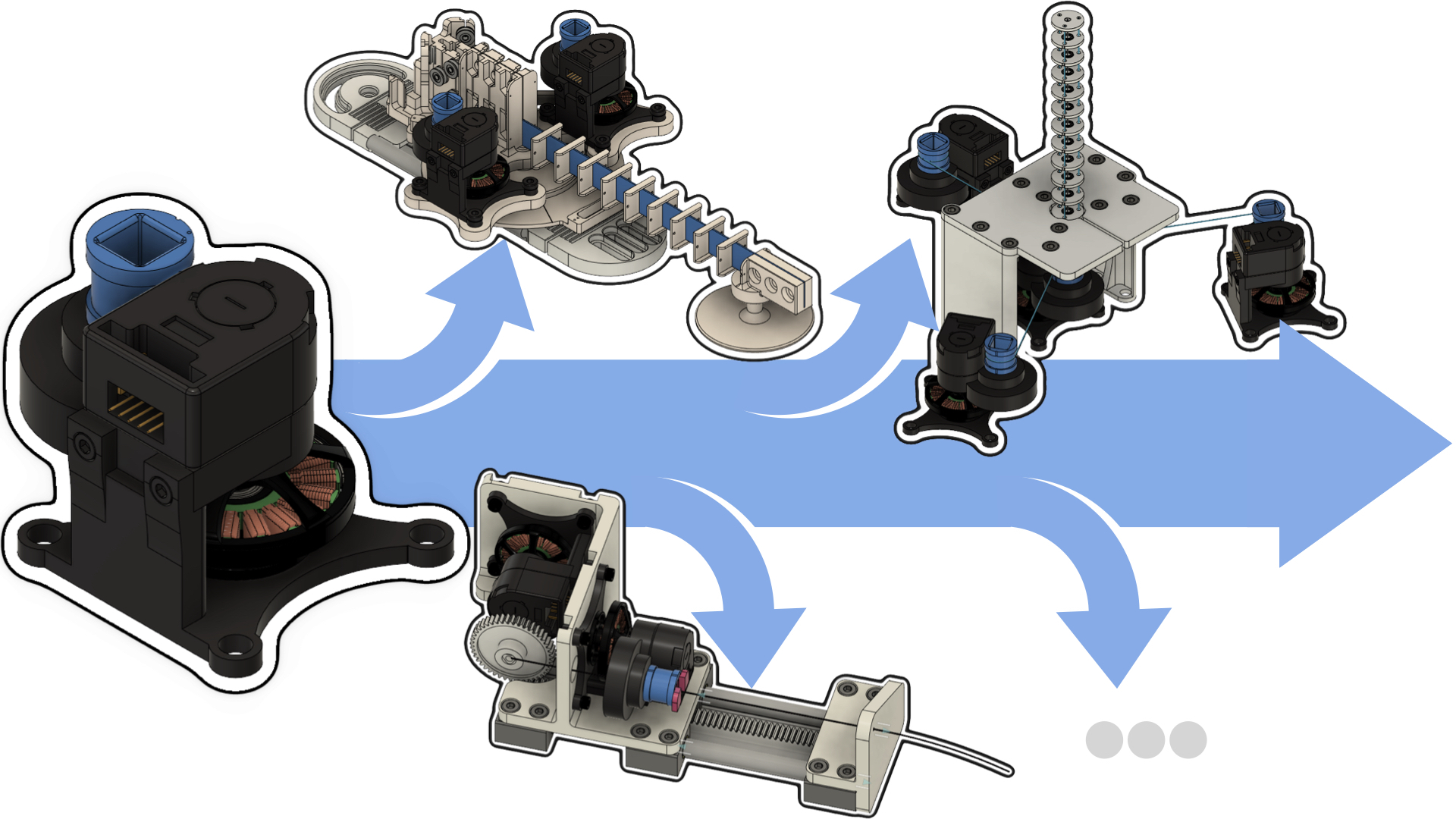
As you are reading this on our blog, you are already aware of our initiative called the OpenCR Project. With this week’s post, we are releasing our open actuation module 1 for the continuum robotics community to build torque-controlled continuum robots. The actuation module is capable of measuring the external torque as demonstrated with very simplified toy examples. Its versatile and modular characteristics are highlighted by building three different types of continuum robot prototypes. The presented prototypes are capable of torque control and fast trajectory tracking making them the first of a kind of the respective continuum robot type.
The Why
Stepping aside, what problem are we actually addressing? In short – the lack of torque-controlled continuum robot prototypes available to all researchers. In fact, this lack is grounded on two observations we made by observing our research community and relating to other research areas in robotics.
First, in our previous study 2, we observed that precious time and focus are devoted to building custom prototypes. One can acknowledge that experiments on physical hardware in robotics are necessary and valuable for evaluations. However, over 60% of all prototypes are used for only a single publication. This demonstrates an inefficient habit of not reusing existing prototypes. Thus, a significant amount of time is devoted to creating proprietary hardware and software. This large and growing number of single-use prototypes imposes a barrier for the research community shifting away time and efforts from important research questions.
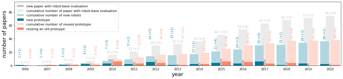
Second, on a more personal note, having the opportunity 3, 4 to regularly work with torque-controlled manipulators such as the Franka Emika Panda5, utilizing torque control for continuum robots seems to be a natural next stepping stone. Torque control has a rich history, especially for serial kinematic mechanisms 6 7 8 5. However, for some reason, the spread and success of torque-control used in pHRI (physical human-robot interaction) research has not reached our continuum robotics community. Perhaps, one reason is that not much time has been directed to build a continuum robot prototype capable of torque control.
The OpenCR Actuation Module
To provide torque-controlled continuum robot prototypes, we propose a modular actuation module consisting of a high-torque brushless electric motor, a high-resolution optical encoder, and a low-gear-ratio transmission. This choice of hardware allows for torque control and fast trajectory tracking in real time. Furthermore, it enables proprioceptive torque sensing by measuring motor currents without relying on additional sensors, e.g., tension sensors or load cells. In addition, the actuation module and its coupling system can be used in different actuation modes for a wide range of continuum robots. For instance, tendon displacement/tension and backbone rotation/torque can be controlled and measured.
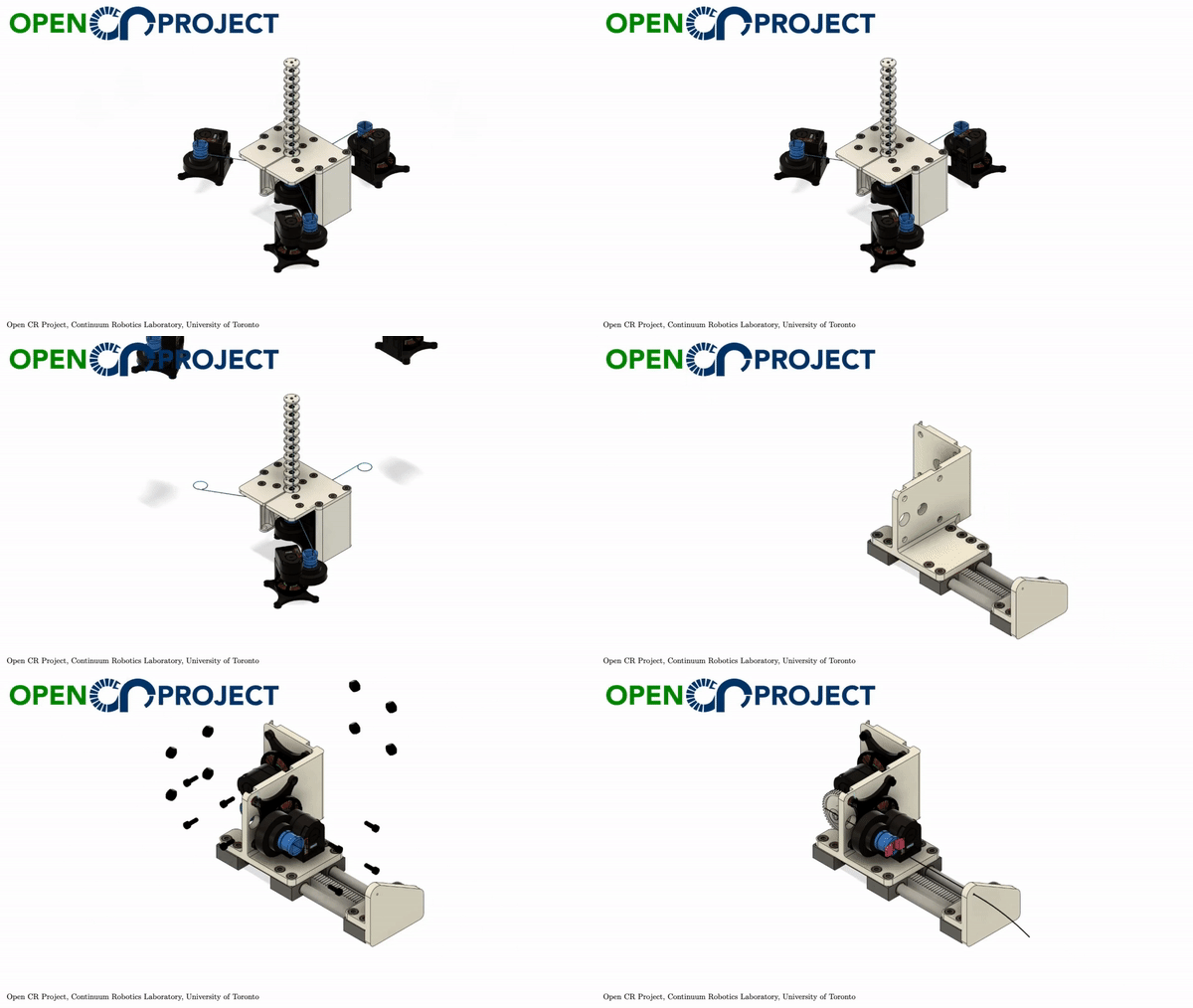
Recapping the technological trend towards torque-controlled robot systems in other research fields, we are forecasting a likely impact of the proposed actuation module and continuum robot prototypes built on it. The manuscript 1 takes initial steps towards advanced control methodologies. We are confident that the ability of continuum robots utilizing our actuation module (or one with similar capabilities) has a decisive advantage over previous existing prototypes. For example, a CTCR can detect external disturbance as shown here:
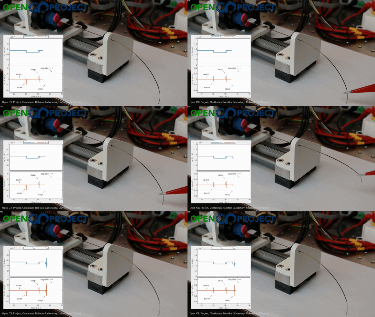
One Actuation Module to Create them All
The actuation module is modular and as such allows you to build any (!?) continuum robot. In the nature of the OpenCR project, we build three different types of continuum robots – a parallel CR, a spatial TDCR, and a CTCR. The image below shows renderings and respective prototypes. By providing open-source hardware and software, we hope that this minimizes the repetitive tasks of developing prototypes, allowing researchers worldwide to focus on the main research challenges in continuum robotics. As a welcome side effect, robot-based evaluations can be performed quickly and become reproducible by other groups!
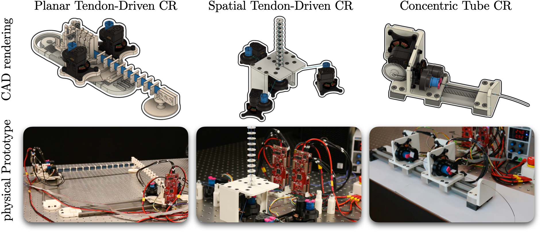
To improve our prototypes, we took great inspiration from the Open Dynamic Robot Initiative, where efforts are made to build cost-efficient actuators for torque-controlled legged robots 9 and manipulators 10. As a matter of fact, open robot hardware projects proliferate progress in robotics 11. Therefore, we encourage you – dear reader – to participate in the development of open-source software and hardware as well as to join the journey of leveraging torque-controlled prototypes. Let’s pave the way with new stepping stones toward untapped or under-investigated research directions.
We hope that the open source nature will bear fruit by opening untapped or under-investigated research directions related to dynamics and advanced control of continuum robots.
References
-
Reinhard M. Grassmann, Chengnan Shentu, Taqi Hamoda, Puspita Triana Dewi, Jessica Burgner-Kahrs. “Open Continuum Robotics – One Actuation Module to Create them All,” 2023, arXiv: 2304.11850 ↩ ↩2 ↩3
-
R. M. Grassmann, S. Lilge, P. Le, and J. Burgner-Kahrs, “CTCR prototype development: An obstacle in the research community?” in Robotics Retrospectives Workshop at RSS, 2020. Online ↩
-
Sami Haddadin, Lars Johannsmeier, Johannes Schmid, Tobias Ende, Sven Parusel, Simon Haddadin, Moritz Schappler, Torsten Lilge, and Marvin Becker. “roboterfabrik: A pilot to link and unify german robotics education to match industrial and societal demands.” International Conference on Robotics and Education, 2018. DOI: 10.1007/978-3-319-97085-1_1 ↩
-
Kristy Strauss, “‘It’s a really cool place’: U of T Mississauga students get hands-on experience in new robotics teaching lab.” Accessed: April 25, 2023 Online ↩
-
S. Haddadin, S. Parusel, L. Johannsmeier, S. Golz, S. Gabl, F. Walch, M. Sabaghian, C. Jaehne, L. Hausperger, and S. Haddadin, “The Franka Emika Robot: A reference platform for robotics research and education,” IEEE Robotics & Automation Magazine, vol. 29, no. 2, pp. 46-64, 2022. DOI: 10.1109/MRA.2021.3138382 ↩ ↩2
-
J. Luh, W. Fisher, and R. Paul, “Joint torque control by a direct feedback for industrial robots,” Transactions on Automatic Control, vol. 28, no. 2, pp. 153–161, 1983. DOI: 10.1109/TAC.1983.1103215 ↩
-
L. E. Pfeffer, O. Khatib, and J. Hake, “Joint torque sensory feedback in the control of a PUMA manipulator,” IEEE Transactions on Robotics and Automation, vol. 5, no. 4, pp. 418–425, 1989. DOI: 10.1109/70.88056 ↩
-
R. Bischoff, J. Kurth, G. Schreiber, R. Koeppe, A. Albu-Schäffer, A. Beyer, O. Eiberger, S. Haddadin, A. Stemmer, G. Grunwald, and G. Hirzinger, “The kuka-dlr lightweight robot arm-a new reference platform for robotics research and manufacturing,” in International Symposium on Robotics, 2010, pp. 1–8. online ↩
-
F. Grimminger, A. Meduri, M. Khadiv, J. Viereck, M. Wüthrich, M. Naveau, V. Berenz, S. Heim, F. Widmaier, T. Flayols, J. Fiene, A. Badri-Spröwitz, and L. Righetti, “An open torque-controlled modular robot architecture for legged locomotion research,” IEEE Robotics and Automation Letters, vol. 5, no. 2, pp. 3650–3657, 2020. DOI: 10.1109/LRA.2020.2976639 ↩
-
M. Wüthrich, F. Widmaier, F. Grimminger, J. Akpo, S. Joshi, V. Agrawal, B. Hammoud, M. Khadiv, M. Bogdanovic, V. Berenz, J. Viereck, M. Naveau, L. Righetti, B. Schölkopf, and S. Bauer, “Trifinger: An open-source robot for learning dexterity,” in Conference on Robot Learning, 2020. arXiv: 2008.03596 ↩
-
V. V. Patel, M. V. Liarokapis, and A. M. Dollar, “Open robot hardware: Progress, benefits, challenges, and best practices,” IEEE Robotics & Automation Magazine, pp. 2–9, 2022. DOI: 10.1109/MRA.2022.3225725 ↩
Why are Continuum Robots predominantly explored for medicial applications?
Looking at the history of continuum robotics, early research has focussed on larger scale continuum robots. Prototypes were built comparable in size to industrial serial arm robots. This probably resulted in expectations in terms of performance. If an industrial robot arm could achieve superior accuracy and repeatabilty with high payloads and at high speed, why would one need a continuum robot performing worse on this scale? Repeatability, accuracy, speed, and payload are clearly not unique selling points for continuum robots. Poised by the third industrial revolution in the late sixties and early seventies of the 20th century, roboticists naturally focussed on robots applicable to automation and its goals. Continuum robots were just not cutting it (yet). Consequently, continuum robotics remained a niche research area for a while.
Medical robotics was just on the onset in the mid eighties and was using repurposed industrial robots. The first medical robotics procedure used the PUMA 560 robot to perform a neurosurgical biopsy at the National Hospital for Neurology and Neurosurgery in London in 1985. The robot guided a needle into the brain to take a tissue sample for examination. Fun fact: The Puma 560 design is based on an earlier robot design by Victor Scheinman, the same Victor Scheinman who developed the first continuum robot.
The trend towards more minimally invasive surgey and ultimatley keyhole access to operate promises benefits for patient care, such as shorter hopsitalization and quicker recovery times. While industrial style robots certainly play an important role in medical robotics today, their large footprint and size naturally places them beside physicians and outside of the patient. But as soon as one wants to move away from large incisions and the need to open the body, thin, versatile, and dextrous robotics enters the scene. Small-scale continuum robots could sneak into a patient with more dextrous motion capabilties than conventional robots and the ability to reach surgical sites inaccessible by conventional robots or standard medical instruments! And that ability is more defining than accuracy and payload. In contrast to industrial automation, small-scale continuum robots promise significant benefit over serial robot arms!
With medical applications, continuum robots found a compelling use case. Motivated by unsought of minimally-invasie approaches and the ability to navigate within the human body through natural orifices or miniscule inscisions, research in continuum robotics excelled. Over the past decades we have witnessed a vast surge in medical continuum robots. In fact, the majority of continuum robot papers draw their motivation from medical applications. The prominent surveys in the field of continuum robotics are centered around medicine1 2 3 and I refer the interested reader to those surveys to learn about the breadth and depth of medical continuum robotics research.
The Untapped Potential
One may argue that continuum robots found their sweet spot in the medical application domain. While this is certainly the case, the untapped potential of continuum robots in non-medical applications is enormous! Think about autonomous small-scale or medium-scale continuum robots in in-situ and non-destructive inspection, maintenance, repair, and operations.
Example: On-wing jet engine inspection provides an example of a keyhole procedure, where a technician inspects components such as turbine blades and the combustion chamber using a flexible camera, called a borescope, through tiny access points on the engine. This is a cumbersome procedure requiring an expert to fiddle with the borescope in hunched body postures, with limited time, as the plane stands ready for takeoff. If an issue is overlooked, e.g., a small crack in a blade, it may be disastrous and result in a worst-case scenario of the engine blowing off during flight. At the same time, full service of an engine means that it must be taken off-wing for maintenance – a costly endeavour. Only very few researcher worldwide look at this problem, with the University of Notthingham spearheading research with Rolls Royce on robotics for in-situ repair
This in-situ inspection is just one of many examples where we can build on our expertise in continuum robotics in the medical domain and innovate the next generation of autonomous continuum robot systems. In fact, non-medical applications for continuum robots are characterized by similar challenges:
- limited accessiblity,
- tortuous pathways in constrained environments, and
- need for dextrous manipulation at the location of interest.
At the same time, turning to new application domains opens new research questions challenging to solve:
- How can we design long continuum robots that can maintain stability?
- How can we avoid buckling for continuum robots navigating cluttered environments?
- How can we achieve dextrous steering and motion capalities and bear sufficient loads?
I envision a new generation of continuum robots that are of small and medium scale, dextrous enough to enter an environment for in-situ inspection, maintenance, and repair through multiple keyholes, which act autonomously and are able to collaborate with one another to achieve the task.
Call to Action
I believe, that we as the continuum robotics community, should turn to non-medical use-cases to invent this next-generation of continuum robot systems with autonomous capabilities. By focussing on medical applications, we have naturally limited our design choices to certain continuum robot dimensions, materials, workspaces, control paradigms, etc. that are informed by anatomical constraints and clinical requirements. In fact, most medical continuum robots are rather short if they can are designed to work in free spaces. Longer medical continuum robots need environmental constraints for steering - such as vasculature for robotic catheters.
Drawing motivation from one application domain lead to narrow thinking and limited creativity. Continuum robotics researchers and innovators have become too focused on the specific needs and constraints of medicine. I argue that this prevented us from considering new and unconventional ideas!
Overall, while focusing on medicine as the dominant application domain was necessary to develop expertise in continuum robotics, it is important for the continuum robotics community to maintain a broad perspective and engage with other fields and industries to encourage innovation and avoid limiting the potential for new and unconventional ideas.
References
-
J. Burgner-Kahrs, D.C. Rucker, and H. Choset: Continuum Robots for Medical Applications: A Survey. IEEE Transactions on Robotics, 31(6), pp.1261–1280. doi: 10.1109/TRO.2015.2489500 ↩
-
T. da Veiga, J.H. Chandler, P. Lloyd, G. Pittiglio, N.J. Wilkinson, A.K. Hoshiar, R.A. Harris, and P. Valdastri: Challenges of continuum robots in clinical context: a review. Progress in Biomedical Engineering, 2(3): 032003, 2020. doi: 10.1088/2516-1091/ab9f41 ↩
-
P.E. Dupont, N. Simaan, H. Choset, and D.C. Rucker: Continuum robots for medical interventions. Proceedings of the IEEE, 110(7):847-870, 2022. 10.1109/JPROC.2022.3141338 ↩