Introduction to Motion Planning for Continuum Robots - Part 1

First though.. What is motion planning?

Motion planning stands as a central pillar in robotics. Planning enables robots and autonomous agents to move themselves and other parts of the world to a desired goal by choosing a sequence of appropriate actions. Like robotics in general, motion planning draws on a number of different fields in developing its tools. Approaches to motion planning have grown out of artificial intelligence, optimal control, and operations research.

That’s the first paragraph of my motion planning course syllabus. It’s a bit… grandiose, but I’ve found it to be effective in convincing the students that they are about to learn something interesting; hopefully it worked on you as well. It was also written by the professor who taught the course before I did, and whose syllabus I used as a starting point for my own (on the shoulders of giants etc etc etc). If that was sufficiently dramatic and you’re convinced to keep reading, let’s get to it.

More colloquially, motion planning can be broadly defined as the problem of computing motions, actions, or controls that move a robot through its environment in such a way that some task is performed while obeying some set of constraints.

In its most basic form, that task can be defined as moving from some start configuration to some goal configuration, with typical constraints being defined as obstacle avoidance over the motion, obeying joint limits, etc. Complexity in task definitions and constraint definitions builds from there.

I personally like to present motion planning as a generic optimization problem and then look specifically at how aspects of that problem are defined. Be forewarned, I’m going to grossly abuse notation/terminology and ignore nuance all over this post with the goal of imparting intuition rather than specifics.

Consider:

$\boldsymbol{\xi}^* = \underset{\boldsymbol{\xi}}{\texttt{argmin}}\ \texttt{cost}(\boldsymbol{\xi})$

$s.t. \ \ \ c(\boldsymbol{\xi}) \ge 0$ $\ \ \ \ \ \ \ \ d(\boldsymbol{\xi}) = 0$

where $\boldsymbol{\xi}$ represents some trajectory, path, or plan parameterization, $\texttt{cost}$ is some cost function defined over these, $\boldsymbol{\xi}^*$ is an optimal plan under the cost function, and $c$ and $d$ are generic, as-of-yet-unspecified inequality and equality constraints (or sets of such constraints).

This generic optimization formalization is sufficiently expressive to talk about most of the basics of motion planning, and by varying how aspects of this formalization are defined we can arrive at most of the ways people have historically thought about motion planning.

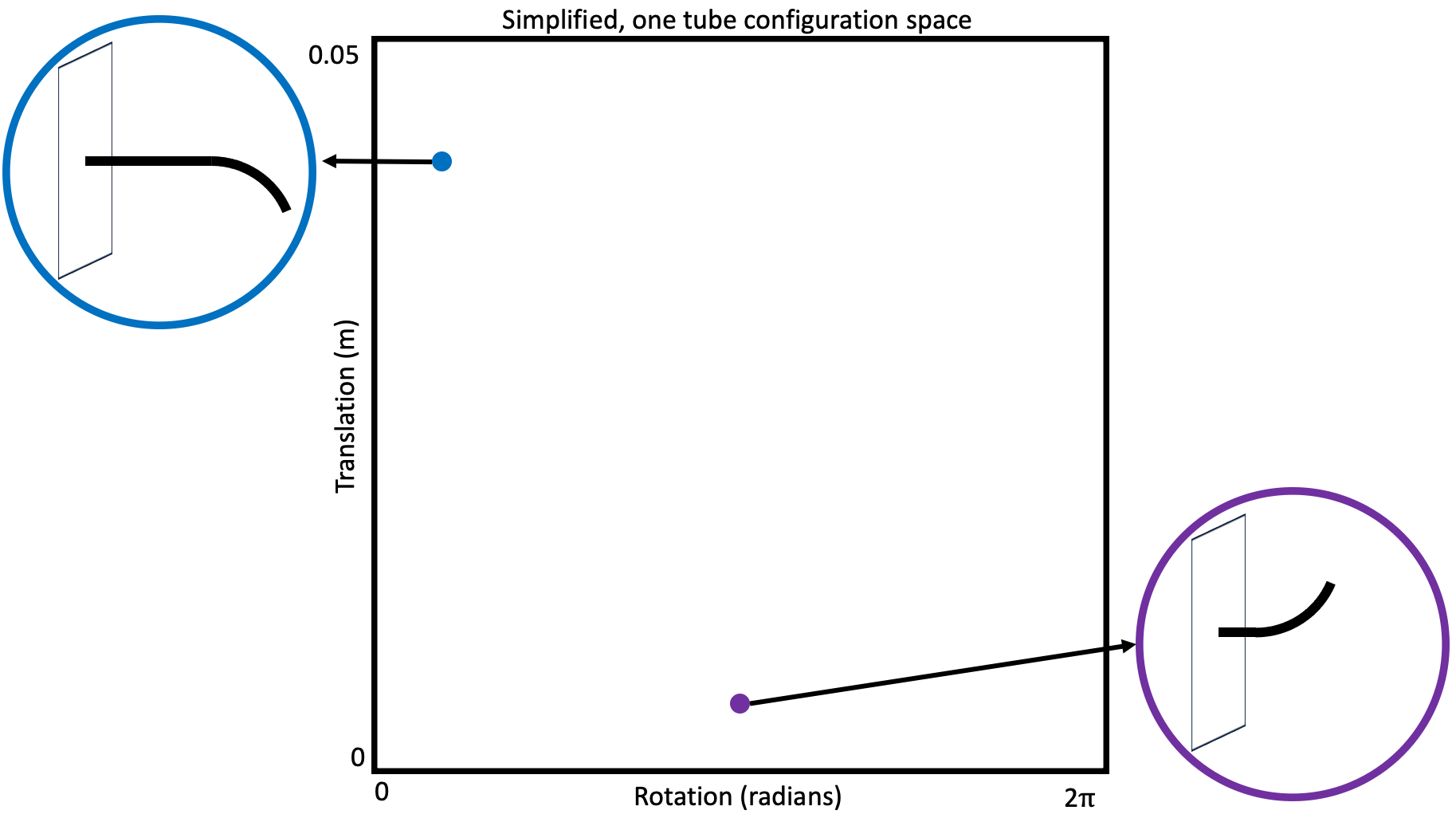
As an example, let’s consider the very simple (relative to other motion planning problems) task of moving a holonomic robot from some start state to some goal state while avoiding some set of obstacles in its environment.

If we conceptualize $\boldsymbol{\xi}$ as defining a space curve in the robot’s configuration space, we can parameterize $\boldsymbol{\xi}$ by the normalized path length such that $\boldsymbol{\xi}(0)$ is the robot’s start configuration and $\boldsymbol{\xi}(1)$ is the robot’s configuration after following the full plan.

Often people consider minimizing path length, so we can imagine defining $\texttt{cost}$ as the length of the path (under some appropriate definition of length).

We also want to constrain the trajectory such that the robot ends in a goal configuration (broadly as an element of some goal set), and such that the entire trajectory avoids obstacles.

We can then cast this simple problem into our optimization framework simply as:

$\boldsymbol{\xi}^* = \underset{\boldsymbol{\xi}}{\texttt{argmin}}\ \texttt{length}(\boldsymbol{\xi})$

$s.t. \ \ \ \boldsymbol{\xi}(0) = \textrm{start configuration}$

$\ \ \ \ \ \ \ \ \boldsymbol{\xi}(1) \in \textrm{goal set}$

$\ \ \ \ \ \ \ \ \boldsymbol{\xi}(s) \textrm{ is collision free } \forall s \in [0,1]$

As in most interesting things, key considerations lie in the details (which I’ve completely ignored above). How is your trajectory parameterized? How do you define your goal set? How do you represent your robot and environment geometry, enabling you to check for collision? Is length even the right objective to minimize? The answer to these questions depends on your specific problem/robot/etc. If I knew what this is for you, I’d just solve your problems myself and take all the credit.

Okay, so this is the first step—representing your problem. Next, let’s solve it.

How do methods typically work?

In my head I broadly group modern motion planning methods into three groups, discrete grid/lattice-based search methods, sampling-based methods, and optimization-based methods. There’s an implied fourth group, “other” or maybe “miscellany”, but I’m going to focus on the first three in this post.

We can parameterize a robot’s configuration space by its actuation variables. Consider here a (ridiculously over-) simplified case of a single-tube concentric tube robot (which makes it just a tube robot, really, nothing concentric about it). We can actuate this robot by translating it in and out of its rectangular base, and by rotating it. A configuration can then be described as a point in this plane where one axis represents the translational value and one the rotational value. In practice, this space will be higher dimensional. For instance, a two-tube concentric tube robot would probably have a 4-dimensional space, two rotational and two translational, and a three-tube robot a 6-dimensional space, etc. It is in this space, which you can think about as the parameterized configuration space, that motion planning frequently happens.

Discrete grid/lattice-based search methods

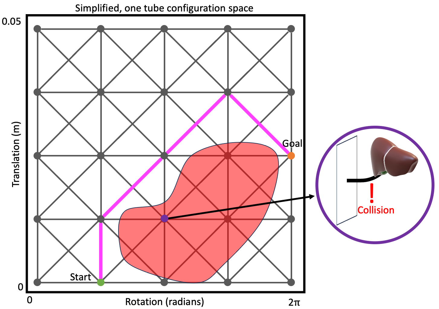
At their simplest, these methods consider a graph or tree (which is just a special kind of graph) embedded in the robot’s configuration space. If you are unsure what I mean by “graph or tree” stop now and read this and this before moving on.

Notably for these methods, the graph is usually implied by a discretization over the robot’s possible actions. Imagine vertices of the graph as representing configurations or states of the robot, and edges as actions between states, which when applied from the source state result in the robot transitioning to the destination state. This action discretization is frequently defined in advance (and you can imagine applying this concept to robot’s with continuous action spaces simply by discretizing those action spaces). Due to the constant discretization, you can conceptualize these as creating something like a grid or lattice as the graph.

With this conceptualization, motion planning then reduces to a search over that graph, seeking the “shortest” path from your start vertex to any vertex that represents a goal configuration or state.

In the discrete grid/lattice-based search methods, we can conceptualize something like this grid-shaped graph embedded in the configuration space. Some of this graph may correspond to configurations where the robot’s shape collides with obstacles, such as this red volume which represents configurations where the tube is colliding with that liver there. (It’s a liver. Don’t ask me where it came from, I don’t make the rules. Regardless, we don’t want to run into it with our robot). If we have a start and goal configuration that are on this graph, or that we can easily connect to this graph, then we can run a graph search algorithm on this graph which, if we do it correctly, will return for us a collision free path (shown here in pink). Note: In these figures I’ve drawn a configuration space obstacle that corresponds to the liver obstacle in the robot’s workspace. This is just an example. This drawing is NOT what the configuration space obstacle would actually look like. In fact, in general it is infeasible to fully describe the configuration space obstacles. Many of the motion planning methods I describe here were designed in part to overcome this very issue.

How does this map back to our optimization formalization above? The cost function is minimized by applying a graph-search method that minimizes the accumulation of edge cost (so you need to define a cost over edges and recognize that without substantial modification you’re limited to considering objectives that can be modeled by costs that accumulate). The constraints are enforced simply by not considering edges that would result in a violation of the constraints during the search.

Cannonical graph search methods (not specific to motion plannning) include Uniform Cost Search (UCS) (closely related to Djikstra’s algorithm) and A* search.

The key to applying these methods in motion planning is frequently in coming up with an effective and admissible/consistent heuristic (see A* details for what that means). More advanced methods applied to motion planning specifically include D*¹, D*-Lite², and LPA*³. It’s also very much worth noting that inadmissible heuristics can also be leveraged to potentially great effect (see Multi-Heuristic A*⁴).

Sampling-based methods

Perhaps the most popular class of motion planning methods, the sampling-based approaches are closely related to the graph-search methods. In fact, these methods frequently leverage graph search but on a graph constructed in a different manner.

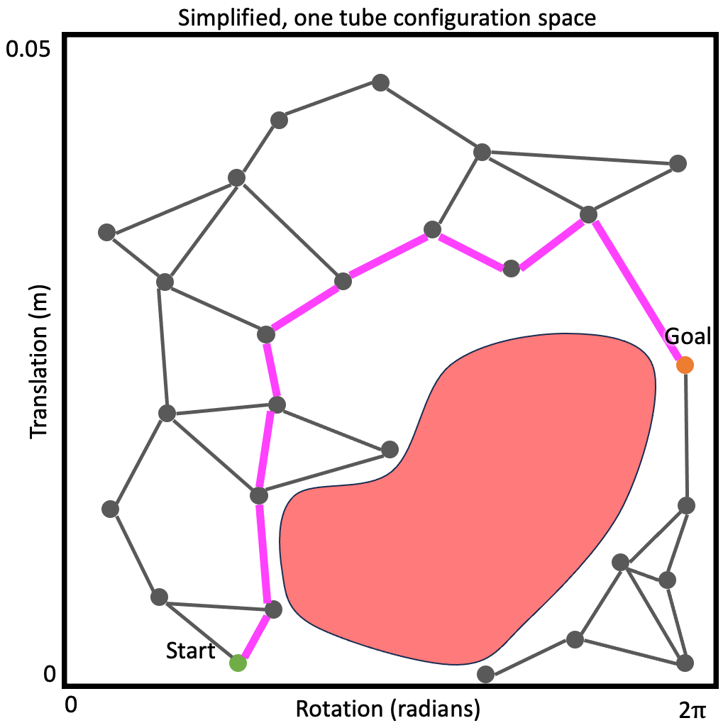
Rather than a graph constructed via a discretization over the robot’s actions, the sampling-based methods leverage random sampling to construct the graph incrementally (this is why they are called sampling-based, as you may have guessed). The graph (or tree, which again, is just a special kind of graph) is embedded in the robot’s configuration space as above. It is constructed by iteratively randomly sampling states (or actions, sometimes) and attempting to connect the newly sampled state (or state resulting from the sampled action) to the graph/tree.

When adding states, (usually) the new state and the edge connecting it to the graph are checked for validity (e.g., joint-limit satisfaction and obstacle avoidance). If the state and/or edge are not valid, they aren’t added to the graph.

At some point, the hope is that the graph will contain a goal state, and then by running graph search (e.g., A*) on this randomly-generated graph the method will find a path from the start state to a goal. If the graph is a tree, this search is trivial as there’s only one path in the graph (ignoring some nuance, that’s what tree means).

In the sampling-based methods, the graph (or tree) is constructed in the configuration space via random sampling. It will almost certainly have a much different structure than the grid/lattice graphs will, and subsequently the algorithms will exhibit different properties.

The specifics of the graph, how the states/actions are sampled, how the connections are made, etc., are what distinguish the sampling-based methods from each other.

Okay, so let’s map these concepts back to our optimization formulation.

Cost: If there are multiple paths in the graph, then the graph search over the graph can provide the lowest cost path in the graph, however the lowest cost path possible may not be in the graph at any given iteration. Many of the earlier versions of these methods ignored cost and instead attempted to find any path that avoided obstacles, providing a property called probabilistic-completeness. Since then, other methods build upon this to provide a guarantee called asymptotic optimality, which intuitively means that their best path will approach an optimal path (in cost) as runtime progresses (only getting arbitrarily close to an optimal path in the limit though). This contrasts with the discrete grid/lattice-based search methods in that those methods typically only provide a property called resolution completeness/optimality which intuitively means the path is complete or optimal for the resolution of the discretization, but not necessarily in general.

Constraints: As with the discrete grid/lattice-based search methods, the sampling-based methods usually encode constraint satisfaction by only considering states/edges in the graph construction or search that satisfy the constraints, including obstacle avoidance.

Canonical probabilistically-complete methods include Probabilistic Roadmaps (PRM)⁵ and Rapidly-exploring Random Trees (RRT)⁶. Popular asymptotically-optimal methods include PRM*/RRT*⁷, Batch-Informed Trees (BIT)⁸, and Asymptotically-Optimal-RRT (AO-RRT)⁹.

Super-duper important point! Just because you’re using sampling-based methods does not mean you’re getting probabilistic completeness or asymptotic optimality. There are properties/assumptions you must satisfy in your specific application of these methods that are frequently nuanced, you’ll need to ensure that you satisfy these things. Read the papers detailing these methods for details!

Optimization-based methods

Given the formulation we started with, i.e., casting the motion planning problem as constrained optimization, you may be asking yourself: “wait, why don’t we just use optimization methods from, you know, mathematics, to solve this problem?” Great question! Enter the optimization-based motion planning methods.

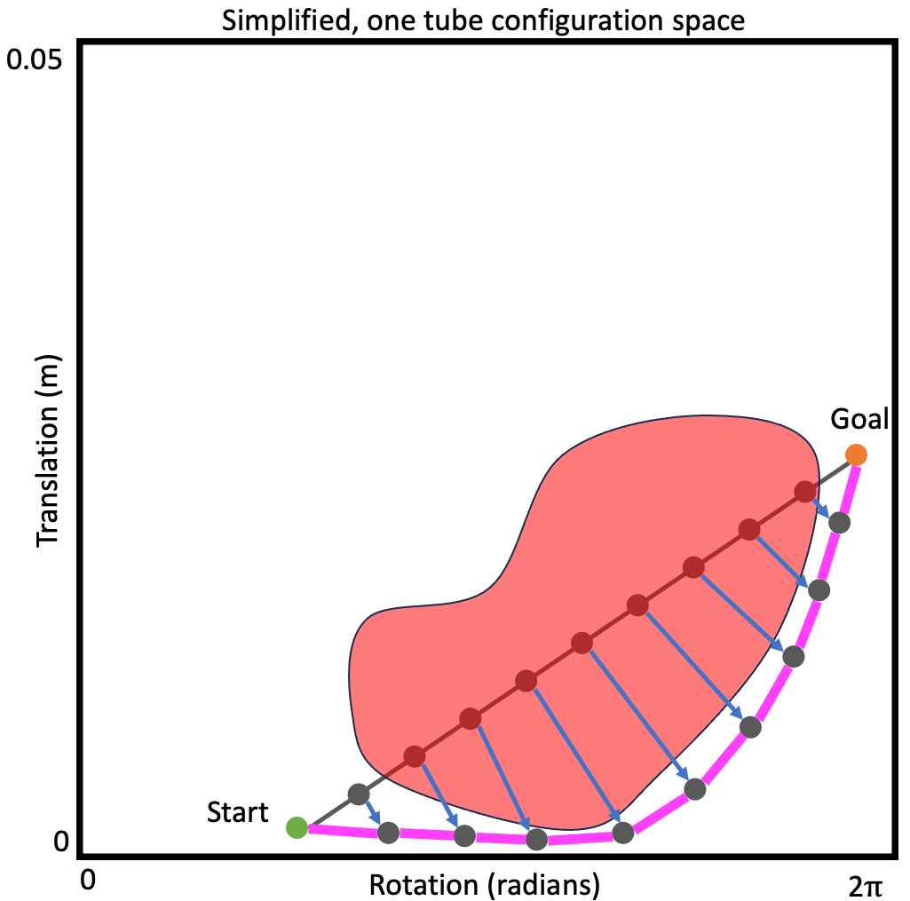
This class of methods leverages nonlinear, constrained optimization methods from the field of optimization itself explicitly to solve the motion planning problem using variations of our above formulation—rather than relying on the graph-search to minimize cost.

As of now, the majority of these methods (with an exception mentioned below) leverage gradients (and frequently higher-order derivatives) of the objective function and/or of the constraint functions in iterative optimization methods. Think penalty methods, augmented Lagrangian methods, interior point methods, etc. If these concepts are new to you, there is an amazing textbook on the subject by Wright and Nocedal ¹⁰ that is open almost perpetually in my office.

At a high level there isn’t much more to the story. These methods take exactly the optimization-based formulation above and apply optimization techniques that work directly on such formulations.

Potentially abandoning the notion of a graph entirely, the optimization-based methods instead frequently parameterize a curve in the configuration space that connects the start and goal. Here that initial parameterization is just an evenly spaced set of configurations in between the start and goal, without consideration of the obstacles. These methods then leverage numerical optimization to minimize an objective while ensuring constraint satisfaction (such as by bringing the path out of regions of the space that collide with obstacles, a process here represented by the blue arrows).

Is it just that easy? Unfortunately, no. The prior paragraph is true at a high level, but the low level is where the details lie. The specific ways in which these methods define cost and their constraint functions such that they work well with the optimization techniques—e.g., ensuring they have gradients that are well-behaved—can make these methods a bit tricky to use in practice. However in many cases they end up working very, very well, which can make it worth the complexity.

Canonical methods include CHOMP¹¹, which leverages a variation of gradient descent, and TrajOpt¹² which leverages Sequential Quadratic Programming (SQP). A different method, that is not nearly as popular as those methods, combines sampling-based planning with interior point optimization¹³. I include it in this list because it was part of yours truly’s PhD work, and so here is a shameless plug.

There is also a method called Cross-Entropy Motion Planning (CEMP)¹⁴ that leverages a gradient-free optimization method (the cross-entropy method, as you may have guessed from the name). This is notable because many difficulties one may encounter in leveraging optimization-based methods may come from the gradients, or lack-thereof.

This concludes Part 1 of my introduction to motion planning for continuum robots. In next week’s Part 2 we will look at the challenges of motion planning for continuum robots. Stay tuned!

References

1. A. Stentz: Optimal and Efficient Path Planning for Partially-Known Environments. IEEE International Conference on Robotics and Automation, pp: 3310–3317, 1994. doi: 10.1109/ROBOT.1994.351061 ↩

2. S. Koenig, M. Likhachev: Fast Replanning for Navigation in Unknown Terrain. Transactions on Robotics, 21(3):354–363, 2005. doi: 10.1109/tro.2004.838026 ↩

3. S. Koenig, M. Likhachev, D. Furcy: Lifelong Planning A*. Artificial Intelligence, 155(1–2):93–146, 2004. doi: 10.1016/j.artint.2003.12.001 ↩

4. S. Aine, S. Swaminathan, V. Narayanan, V. Hwang, M. Likhachev: Multi-heuristic A*. The International Journal of Robotics Research, 35(1-3): 224-243, 2016. doi: 10.1177/0278364915594029 ↩

5. L.E. Kavraki, P. Svestka, J.C. Latombe, M.H. Overmars: Probabilistic roadmaps for path planning in high-dimensional configuration spaces. IEEE Transactions on Robotics and Automation, 12(4):566-580, 1996. doi: 10.1109/70.508439 ↩

6. S.M. LaValle and J.J. Kuffner Jr: Randomized kinodynamic planning. The International Journal of Robotics Research, 20(5):378-400, 2001. doi: 10.1177/02783640122067453 ↩

7. S. Karaman and E. Frazzoli: Sampling-based algorithms for optimal motion planning. The International Journal of Robotics Research, 30(7):846-894, 2011. doi: 10.1177/0278364911406761 ↩

8. J.D. Gammell, T.D. Barfoot, S.S. Srinivasa: Batch Informed Trees (BIT*): Informed asymptotically optimal anytime search. The International Journal of Robotics Research, 39(5):543-567, 2020. doi: 10.1177/0278364919890396 ↩

9. K. Hauser, Y. Zhou: Asymptotically optimal planning by feasible kinodynamic planning in a state–cost space. IEEE Transactions on Robotics, 32(6):1431-1443, 2016. doi: 10.1109/TRO.2016.2602363 ↩

10. J. Nocedal and S. Wright: Numerical optimization. Springer-Verlag New York, 2006. doi: 10.1007/978-0-387-40065-5 ↩

11. M. Zucker, N. Ratliff, A.D. Dragan, M. Pivtoraiko, M. Klingensmith, C.M. Dellin, J.A. Bagnell, S.S. Srinivasa: Chomp: Covariant hamiltonian optimization for motion planning. The International Journal of Robotics Research, 32(9-10):1164-1193, 2013. doi: 10.1177/0278364913488805 ↩

12. J. Schulman, Y. Duan, J. Ho, A. Lee, I. Awwal, H. Bradlow, J. Pan, S. Patil, K. Goldberg, P. Abbeel: Motion planning with sequential convex optimization and convex collision checking. The International Journal of Robotics Research, 33(9):1251-1270, 2014. doi: 10.1177/0278364914528132 ↩

13. A. Kuntz, C. Bowen, R. Alterovitz: Fast anytime motion planning in point clouds by interleaving sampling and interior point optimization. Robotics Research: The 18th International Symposium ISRR, pp. 929-945, 2019. doi: 10.1007/978-3-030-28619-4_63 ↩

14. M. Kobilarov: Cross-entropy motion planning. The International Journal of Robotics Research, 31(7):855-871, 2012. doi: 10.1177/0278364912444543 ↩