Introduction to Motion Planning for Continuum Robots - Part 2

Today, we continue our introduction to motion planning for continuum robots. If you have missed Part 1 of the intro, look at last week’s blog post before you continue here!

What makes motion planning particularly challenging for continuum robots?

First, let’s discuss one of the primary differences between continuum robots and more “traditional” robots (for lack of a better term)—modeling.

As you’ve seen in prior (and future, I promise) blogs on this site, modeling the mechanics of continuum robots is fundamentally different from more traditional serial-link manipulator arms.

As a subset of mechanics, consider just the forward kinematics (FK) problem for continuum robots, i.e., mapping the robot’s joint state to the robot’s resultant shape in space. For concentric tube robots this may be mapping the robot’s tubes’ rotation/translation values to the robot’s shape and for tendon-driven robots this may be mapping the robot’s tendon tensions/displacements to the robot’s shape.

What’s actually happening in the physical world is complicated here. There are elastic elements interacting with (potentially) other elastic elements in complex ways. There is difficult-to-model friction between components of the robot, hysteresis, potentially difficult-to-predict material properties, etc.

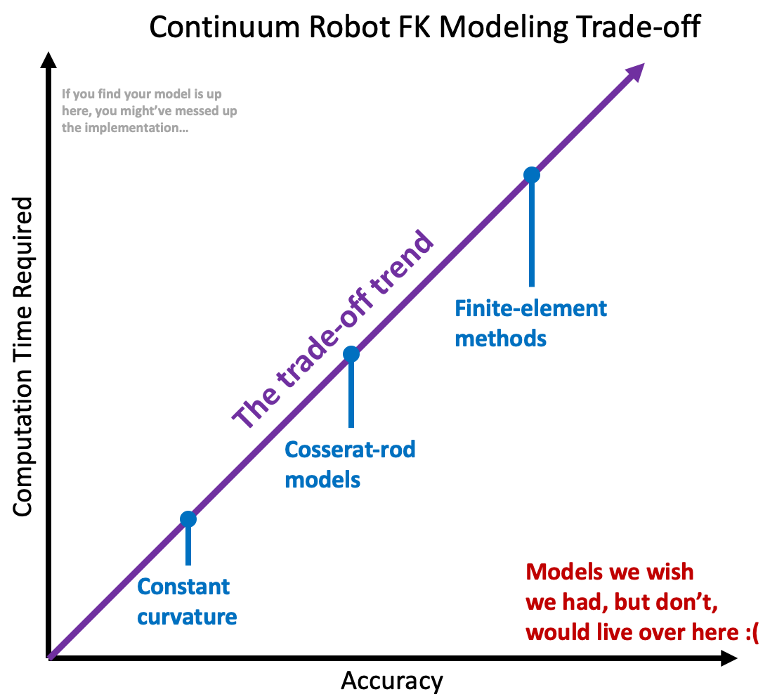
The continuum robotics community has taken a variety of approaches to modeling, but a fundamental trend exists: a trade-off between accuracy and speed-of-computation. That is, models which may be fast to compute are typically fast because they neglect to account for some of the physical phenomenon present in the actual robot. On the flip side, models that account for those phenomenon are slow to compute. In reality, there’s a spectrum here.

Constant curvature models, for instance, may take a purely geometric approach to FK, which is fast to compute, but tend to be less accurate. On the other end of the spectrum, you could consider leveraging something like finite element analysis to simulate the physics of a continuum robot to compute its shape. This would improve accuracy but would be much, much slower to compute. Somewhere in the middle of these you may find things like the Cosserat rod/string models, which are a popular way to model continuum robots and will be discussed in other blog posts here (this is the approach we take in my lab, usually, when we aren’t using machine learning-based methods).

Let’s contrast this with serial-link manipulator arms. For these, FK typically require only the multiplication of a handful of matrices, which is comparatively VERY fast, and comparatively VERY accurate, as these robots are rigid.

Okay, so why is this a problem when performing motion planning for continuum robots?

Well, one way to think about motion planning is that we are reasoning in advance of actually moving about the best way to move the robot to achieve our goals. This means that we need our ability to reason about motion to be accurate, otherwise how we predict the robot will move doesn’t mean much. For this reason, model inaccuracy plays havoc with naïve motion planning methods (such as we’ve discussed in last week’s post), and continuum robots have inaccurate models.

Further, the ways in which we are reasoning in advance about moving require us to consider a whole bunch of potential motions for the robot. Every vertex in the grid/lattice-based and sampling-based methods represents an FK computation. Every edge between them requires multiple (often many) FK computations. In the optimization-based methods, the computation of objective and constraint gradients frequently require many FK computations. So the time it takes to compute FK has HUGE implications in motion planning.

This modeling tension, fast but inaccurate or (somewhat) accurate but slow, is one of the fundamental challenges of applying motion planning to continuum robots, and the one I’ll focus on for the rest of this post.

As continuum robot models become more accurate, they tend to take longer to compute. This represents one of the fundamental challenges associated with applying motion planning to continuum robots.

How has the community overcome these challenges?

Modeling accuracy (or lack thereof)

The continuum robotics community (myself included) has largely taken an extremely unsatisfying approach to overcoming modeling inaccuracy. This approach, also used by much of the non-continuum robotics planning world, boils down to a simple idea: don’t let the robot get close to things. That way, if the model is inaccurate, hopefully the robot is far enough away from its environment that it won’t collide with it in unexpected ways.

As an example, in one of my papers¹, we build into the objective function a notion of distance from obstacles. Specifically, We define the cost of a configuration $\boldsymbol{q}$ as:

\[\begin{split} &\texttt{cost}(\boldsymbol{q})=\left\{ \begin{array}{rcl} \cfrac{1}{\texttt{clear}(\boldsymbol{q})},&&\texttt{clear}(\boldsymbol{q}) > 0\\ \infty,&&\texttt{clear}(\boldsymbol{q}) \le 0, \end{array}\right. \end{split}\]

where $\texttt{clear}$ is, informally defined here, the signed distance from the robot’s body at that configuration to the nearest obstacle.

The cost of a path $\boldsymbol{\xi}$ then becomes \(\texttt{Cost}(\boldsymbol{\xi}) = \int_0^1 \texttt{cost}(\boldsymbol{\xi}(s))ds .\)

where $s$ is a normalized path arclength parameter. Note here that I’ve used little ‘c’ cost for cost over configuration and big ‘C’ Cost for cost over a path. Creative, I know.

You should really read the paper if you want formality here, but this should give you the gist. Also note that in the paper the notation is slightly different, but I’ve changed it here to more-closely match what I’ve used in the last post.

In that method, we leverage both sampling-based motion planning and optimization-based motion planning in parallel (building on [13]), where the method attempts to minimize the $\texttt{cost}$ of a path. This results in paths that travel as far from obstacles as possible, while still being constrained at the start and end configurations.

Computation speed (or lack thereof)

The community has taken a variety of approaches to overcome the slow computation speed of continuum robot mechanical models. Here are a few, with some examples.

The first, and most obvious, is the use of a fast-but-inaccurate mechanical model: For instance, in Lyons et al. ², the authors simplify the mechanical model of concentric tube robots in two key ways. First, they assume that the tubes are torsionally rigid. Second, they assume that the stiffness of each tube dominates all of the tubes nested inside of it. This means that the shape of a tube is assumed to be independent of the motions of the tubes internal to it and that each tube deploys in a constant-curvature circular shape. The mechanical model that leverages these assumptions is sufficiently fast for planning, but again as discussed above ad nauseam, comes at the significant cost of accuracy.

Another approach is to lean on advances in software engineering and programming languages to speed up the computation: Leibrandt et. al.³ leverage template metaprogramming in C++, which (I’m oversimplifying this explanation) moves a lot of expensive run-time computation to compile-time computation for concentric tube robots. This enabled very fast kinematics computation. The method leverages this in a PRM-style motion planner. In our paper¹ mentioned above, we use this template-based kinematic model, wrapping our parallel sampling and optimization method around it. Speaking of, our¹ use of parallelism is another example of leveraging software engineering concepts to speed up computation in planning for continuum robots.

We can also consider leveraging precomputation: In the paper ⁴ (its extension ⁵), the authors propose leveraging precomputation to build a roadmap for planning after the environment is known but in advance of when it is needed. This is a pretty specific (and restrictive) scenario, but makes sense in the application put forth by the papers, namely in surgery. These works present the case that pre-operative medical imaging provides the method with a 3D environment a day (or more) prior to when the surgery will happen. The method can then leverage that time to compute a dense, collision-free roadmap before it’s needed at surgery time. The proposed method utilizes the sampling-based method Rapidly-exploring Random Graph (RRG) (which is also presented in ⁶, in addition to PRM* and RRT*). The method also utilizes one of, if not the most precise (at the time, at least) mechanical models available for concentric tube robots. This dense, collision-free roadmap is built over the course of many hours using this accurate model and the anatomical environment segmented from the pre-operative medical imaging. Then, at the time of the surgery, the method proposes an interactive-rate supervisory control-style scheme in which a haptic device is used by the surgeon to input a desired tip position for the robot in the patient. Leveraging a nearest-neighbor data structure, the vertex in the roadmap that corresponds to the configuration with the robot’s tip closest to the desired position is then identified. Graph search is performed to identify a path on the roadmap from the current configuration to that configuration, and then the method “steps off” of the roadmap and leveraging damped least-squares iterative inverse kinematics ⁷⁸, which is conceptually very similar to resolved-rates control, drives the tip of the robot as close to the desired tip position as it can. This then repeats in a loop.

In our paper⁹, my group has built upon this concept in a few ways. Among other contributions, we adapt the concepts to work for tendon-driven continuum robots (⁴ and ⁵ are specific to concentric tube robots), introduce a modification to mechanical modeling and collision detection to improve speed, and remove the need to have the environment in advance of precomputing the dense roadmap. The method still heavily leverages precomputation, but only requires the environment immediately prior to when the supervisory control loop is started.

So what’s next?

What are the open problems or areas to be explored in motion planning for continuum robots? Here are a few that I’m personally excited about.

Leveraging learned models in planning

There has recently been a large interest in machine learning-based mechanical models of continuum robots, both for their potential to learn unmodeled (or unknowable/unmodelable) effects and their potential for fast computation (e.g., frequently the shape computation of a learned model is faster than the physics-based equivalent). I’ll leave the details of these methods to another post, written by myself or someone else. However germane to THIS post, how to leverage these types of models for motion planning of continuum robots is as-yet underexplored.

Principled planning under uncertainty

Motion planning in a way that handles uncertainty in a principled way has been leveraged to great effect in other areas of robotics. Given the uncertainty associated with continuum robots, the application/exploration of using these types of methods/formulations in planning for continuum robots has great potential.

Multi-fidelity planning

The fact that we have a variety of models for continuum robots that trade computation speed for accuracy implies exciting potential for the use of multi-fidelity planning. One can imagine, as maybe the most obvious example, using a fast but inaccurate model to prioritize edge evaluation in a lazy planning paradigm, look up Lazy PRM if that doesn’t make sense to you, where full edge evaluation is then done with a high-fidelity model.

Closing remarks

Hopefully the above alongside last week’s Part 1 were a relatively gentle introduction to motion planning and how it relates conceptually to continuum robots. This wasn’t intended to be a comprehensive survey of planning for continuum robots. Rather, my intention was to give you the vocabulary and an understanding of the rough concepts sufficient for you to investigate the rest of the literature yourself, and to innovate on the state-of-the-art as you need for your specific problems.

References

1. A. Kuntz, M. Fu, R. Alterovitz: Planning High-Quality Motions for Concentric Tube Robots in Point Clouds via Parallel Sampling and optimization. IEEE/RSJ International Conference on Intelligent Robots and Systems (IROS), pp. 2205-2212, 2019. doi: 10.1109/IROS40897.2019.8968172 ↩ ↩² ↩³

2. L. A. Lyons, R. J. Webster, R. Alterovitz: Motion planning for active cannulas. IEEE/RSJ International Conference on Intelligent Robots and Systems, pp. 801-806, 2009. doi: 10.1109/IROS.2009.5354249 ↩

3. K. Leibrandt, C. Bergeles, G.-Z. Yang: Concentric Tube Robots: Rapid, Stable Path-Planning and Guidance for Surgical Use. IEEE Robotics & Automation Magazine, vol. 24, no. 2, pp. 42-53, 2017. doi: 10.1109/MRA.2017.2680546 ↩

4. L. G. Torres, C. Baykal, R. Alterovitz: Interactive-rate motion planning for concentric tube robots. IEEE International Conference on Robotics and Automation (ICRA), pp. 1915-1921, 2014. doi: 10.1109/ICRA.2014.6907112 ↩ ↩²

5. L. G. Torres et al.: A motion planning approach to automatic obstacle avoidance during concentric tube robot teleoperation. IEEE International Conference on Robotics and Automation (ICRA), pp. 2361-2367, 2015. doi: 10.1109/ICRA.2015.7139513 ↩ ↩²

6. S. Karaman and E. Frazzoli: Sampling-based algorithms for optimal motion planning. The International Journal of Robotics Research, 30(7):846-894, 2011. doi: 10.1177/0278364911406761 ↩

7. Y. Nakamura and H. Hanafusa: Inverse Kinematic Solutions With Singularity Robustness for Robot Manipulator Control. ASME. J. Dyn. Sys., Meas., Control., 108(3):163–171, 1986. doi: 10.1115/1.3143764 ↩

8. C. W. Wampler: Manipulator Inverse Kinematic Solutions Based on Vector Formulations and Damped Least-Squares Methods. IEEE Transactions on Systems, Man, and Cybernetics, 16(1):93-101, 1986. doi: 10.1109/TSMC.1986.289285 ↩

9. M. Bentley, C. Rucker, A. Kuntz: Interactive-Rate Supervisory Control for Arbitrarily-Routed Multitendon Robots via Motion Planning. IEEE Access, vol. 10, pp. 80999-81019, 2022. doi: 10.1109/ACCESS.2022.3194515 ↩