
Open Source FTL Motion Planner
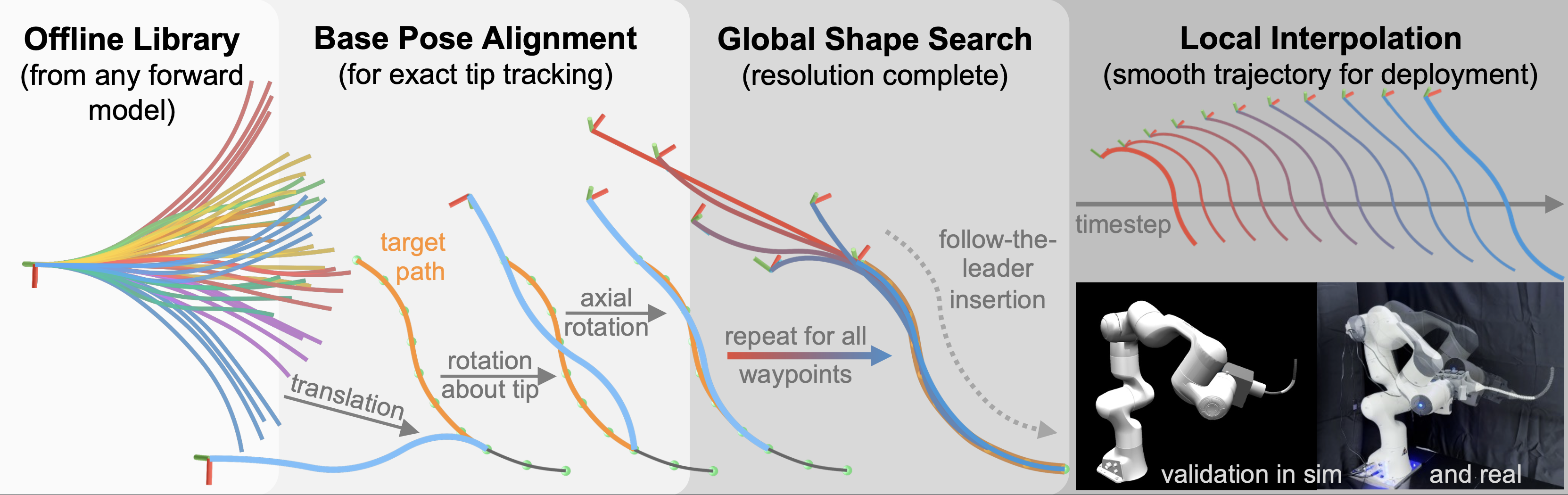
Follow-the-leader (FTL) motion exploits the unique morphology of continuum robots to navigate confined spaces by having the body retrace the path of the tip. We have developed a new approach to achieve FTL motion with a sampling-based motion planner that jointly considers robot configuration and base pose. The key idea is to decouple global shape search from base pose determination by computing the base pose through a closed-form geometric construction, thereby avoiding iterative optimization during online planning. The approach supports general forward models and enables efficient planning by shifting the majority of computation offline. As part of our OpenCR project, We have open sourced the code and planner used in the paper. Additional implementation details can be found in the paper. We also set up an interactive demo on our project website where you can run the planner in the browser here.
In this post, we present a tutorial on how to use our open source sb-ftl-cr-planner codebase. With our implementation, you can define a 3D curve and execute our motion planner to perform FTL motion along the curve. The planner is implemented in Python and uses Matplotlib for visualization.
Problem Defintion
FTL motion is roughly characterized by having the CR body follows the path traced by its tip during insertion 1. The desired path is given as an order set of 3D waypoints \(\mathcal{W}=\{\mathbf{w}_1, \mathbf{w}_2, ..., \mathbf{w}_n\}\). To formalize the requirments of FTL motion, we define two properties that should hold throughout the trajectory.
- \(\textbf{Tip tracking}:\) The tip should be placed at waypoint \(\mathbf{w}_i\) when passing through it, and follow a smooth interpolation (e.g, linear) between consecutive waypoints.
- \(\textbf{Shape following:}\) The inserted portion of the robot should minimize deviation from the corresponding segment of the path.
We consider a CR mounted to a 6-DOF base, representing practical systems where CRs are attached to serial manipulators. The CR configuration space is denoted by \(\mathcal{Q} \in \mathbb{R}^d\) and the combined system configuration space is \(\mathcal{K}=SE(3)\times\mathcal{Q}\). The goal of a FTL motion planner is to generate a sequence of \(N\) configurations \(\{(\mathbf{T}_{b,1}, \mathbf{q}_1),...,(\mathbf{T}_{b,N}, \mathbf{q}_N)\}\) that guides the robot through the path \(\mathcal{W}\) while obeying the two listed properties above.
Code Organization
The planner can be ran in headless mode or with a visualizer using Matplotlib. Installation instructions can be found in the README here. Three core classes are utilized in this repository.
Robot Class
The robot class ContinuumRobotModel(num_segments, segment_lengths, tendon_offset, *args, **kwargs) contains necessary helper functions used throughout the planner. Notable is the forward_kinematics(clark_coordinates: np.ndarray) which returns an array of points along the robot backbone. Forward kinematics is left as an abstract unimplemented method in the parent class. Our planner is model agnostic meaning any forward model (e.g, Constant Curvature, Cosserat Rod, Simulation) can be used. We provide a ConstantCurvature(*args, **kwargs) child class that implements the forward kinematics based on the the constant curvature model. To add in your own model, all you have to do is inherit the parent ContinuumRobotModel class and implement your own forward kinematics function.
Motion Planner Class
The FTL motion planner is implemented as inherited classes of the parent class GeneralMotionPlanner(*args, **kwargs). Similar to the robot class, it contains helper functions with the follow_path() function to be implemented in child classes. We provide 3 planners
No Cluster/Linear SamplingThreshold ClusterDirect Optimization
which all inherit the parent GeneralMotionPlanner class. Each have their own implementation of follow_path() and discussed further in the paper.
Desired Curve Class
To define the desired path for the CR to follow, the TaskGenerator(*args, **kwargs) class is used. Once initialized, this class has many methods to generate 3D curves. Some of the provided curves are,
- Quadratic bezier curve:
generate_curved_path() - Cubic bezier curve:
generate_cubic_bezier_path() - Circular arc:
generate_c_shape_path() - Straight zig-zag:
generate_z_shape_path() - Spiral curve:
generate_spiral_path()
This list is not exhaustive, but if nothing fits your use case, feel free to define your own custom path. As long as the curve is a numpy array of 3D points, our planner can follow it!
Code Walkthrough
We will now walkthrough the provided starter script run_example.py. You can do a quick run with
python run_example.py
or use any of the provided command line arguments (python run_example.py --help). A few useful variations are,
# Linear-search baseline on an S-shape, 20k library, no animation
python run_example.py --planner "No Cluster/Linear Sampling" --curve s \
    --num-samples 20000 --no-animate

# Use an externally produced shape library (skips library generation)
python run_example.py --shape-lib-path /path/to/library.json

# Save the dense motion plan (Clarke coords + base SE(3) + shape per step) to JSON
python run_example.py --save-history my_plan.json
First, the robot model is initialized with the desired system parameters.
robot = ConstantCurvature(
    num_segments=3,
    segment_lengths=[1, 1, 1],
    tendon_offset=[0.2, 0.2, 0.2],
    points_resolution=0.05,
)
After the robot is created, we define the desired path using the provided helper function and command line arguments,
generator = TaskGenerator(robot)
waypoints = _build_curve(generator, args.curve, args.num_waypoints, p1=args.p1, p2=args.p2)
by default, a quadratic bezier curve is created,
generator.generate_curved_path(
    np.array([0, 0, 0]),
    np.array([2, 0, 1.3]),
    np.array([0, 0, 1.6]),
    num_waypoints=num_waypoints,
)
Now it is time to create the shape library! The high dimensioal configuration space of \(\mathcal{K}\) and nonlinear CR dynamics make iterative optimiztion approaches computationally exspensive. Generating a shape library offline then performing global shape search is the technique that makes our method Model agnostic, Efficient and Theoretically Guaranteed. These benefits are discussed more in the paper.
general_follower = GeneralPathFollower(robot)
sampler = general_follower.get_sampling_methods_by_name([args.planner])[0]
...
follower = sampler(**sampler_kwargs)
Initalizing the sampler class generates the shape library using the provided robot object and saves the library as an attribute.
Generating a Shape Library:
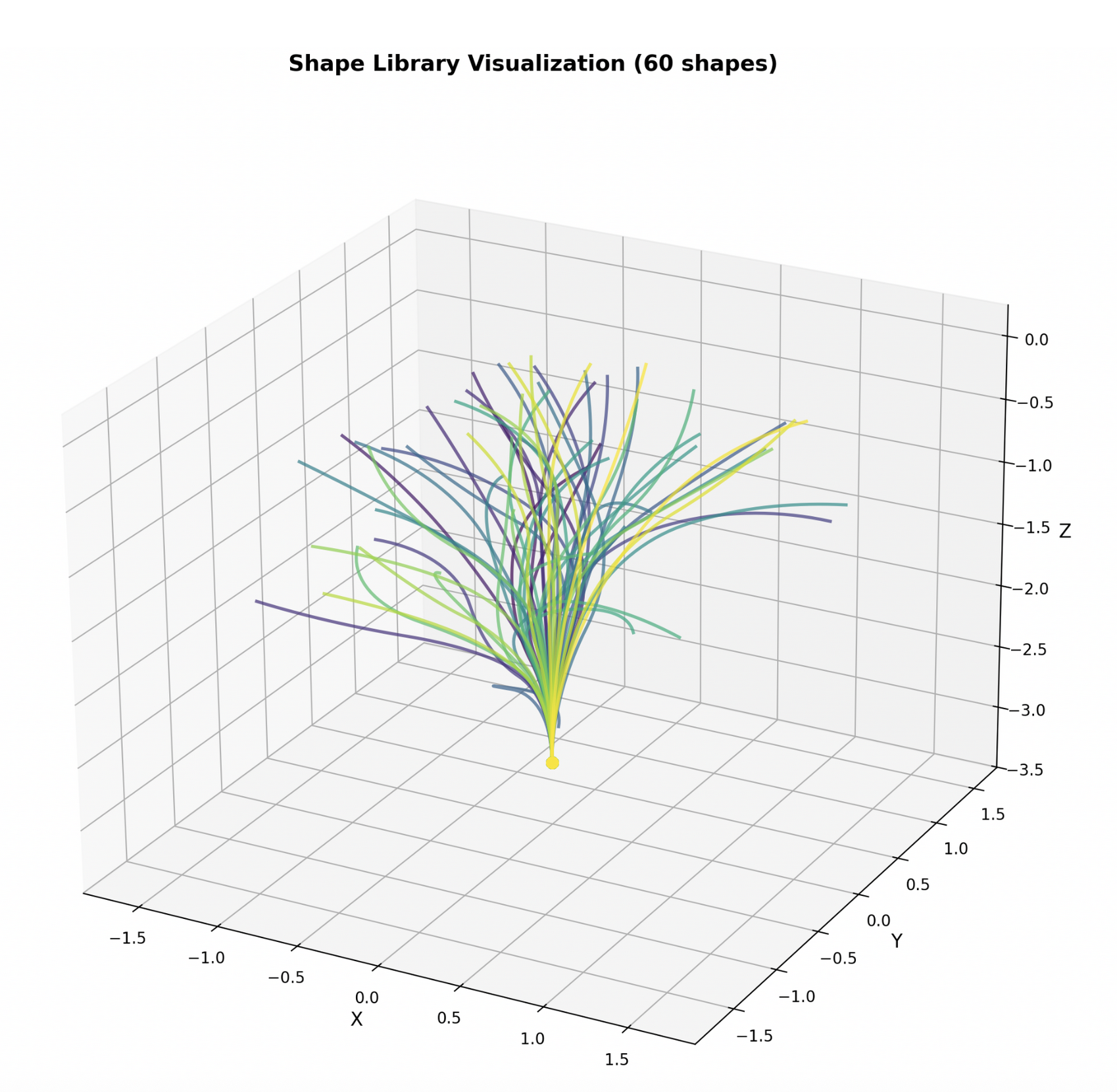
A core feature of our motion planner is that the shape library can be generated offline and reused. This enables the ability to generate very large or computationally exspensive libraries with complex models beyond just Constant Curvature once, and not have it effect the runtime of the planner. In run_example.py we generate a fresh library on each run as the cost for generation with the ConstantCurvature forward model is low and takes less than 30 seconds with 20,000 shapes.
Here is a visualization of 60 shapes from a shape library,
Finally, lets Follow-The-Leader!
history = follower.follow_path(waypoints)
interp_history, interp_waypoints = general_follower.interpolate_mp(
    history, steps_per_waypoint=args.interpolation_steps, enable_optimization=True
)
follow_path() generates the sparse motion plan, one configuration \((\textbf{T}_{b, i}, \textbf{q}_{i})\) for each waypoint \(\mathbf{w}_i\) while interpolate_mp() fills in the gaps between each waypoint by intelligently interpolating between each configuration from follow_path().
Once the motion plan is created, we include support to record deviation statistics and save the motion plan to disk.
Matplotlib is used to visualize the motion plan,
visualizer = PathVisualizer(robot)
visualizer.plot_history(history, waypoints, show_animation=True)
visualizer.plot_history(interp_history, waypoints, show_animation=True, animation_interval=0.01)
both the sparse motion plan and interpolated motion plan are animated. The animation for the sparse plan (left) and interpolated plan (right) are shown below.
Happy tendon-driven continuum robotic simulating!
References
-
Maria Neumann and Jessica Burgner-Kahrs. Considerations for follow-the-leader motion of extensible tendon-driven continuum robots. IEEE International Conference on Robotics and Automation, pages 917–923, 2016. doi: 10.1109/ICRA.2016.7487223 ↩